This article will assume some familiarity with narrow phase collision detection methods and associated geometric concepts such as the Minkowski sum.

A few years ago I was watching Dirk’s great presentation, The Separating Axis Test between Convex Polyhedra (video, slides). Around the 18 minute mark (slide 29) he starts talking about overlaying Gauss maps of convex polyhedra to find the faces of their Minkowski difference.

The upshot is that all faces of the minkowski difference are either:

1. A face of shape A

2. A face of shape B

3. A cross product of an edge from A and an edge from B

And most importantly, you can avoid a costly full support function evaluation in case #3 because you know a vertex that lies on the face. After letting that fact sink, I wondered — why can’t we skip the support function evaluation for all the points on the Gauss map? Turns out you can, the result is a version of the separating axis test that requires only one full support function evaluation as opposed to FaceCountA+FaceCountB. Before we get to the details, let’s back up a bit.

TLDR: Github repo

Collision Detection Formalization

Let A and B be two bounded convex sets in R³. There are two scenarios:

1. No overlap — We want the closest point between the two sets.

2. Overlap — We want to find the minimum translation we can apply to separate the shapes.

Let’s describe each case more formally and discuss solvers that are appropriate.

No Overlap Case

Suppose A and B are disjoint sets. The closest pair of points, one from each set, is the pair that minimizes the distance between them. The following formulations are equivalent.

1) 
   minx,y |x-y|^2 
   x ∈ A
   y ∈ B

2) 
 = minx,y d   
   d ≥ |x-y|^2
   x ∈ A
   y ∈ B

3)
 = mind,z d       
   d ≥ |z|^2
   z ∈ A-B
 

Notice that the Minkowski difference shows up in the last formulation. Since all of these formulations are convex, iterative convex solvers should quickly converge to the global solution. A discussion of non-GJK solvers in games deserves its own post. For the rest of this one, I’ll focus on the overlapping case.

Overlap Case

Suppose A and B are intersecting. To push the sets apart we must find a direction v and a distance s such that the translated set (B+s*v) has no intersection with A.

5) 
   mins,v s
   |v| = 1
   (y+s*v) • v ≥ x • v, ∀x ∈ A, ∀y ∈ B
    
6) 
 = mins,v s
   |v| = 1
   (y-x) • v ≥ -s, ∀x ∈ A, ∀y ∈ B

7) 
 = mins,v s
   |v| = 1
   z • v ≤ s, ∀z ∈ A-B

8) 
 = mins,v s
   |v| = 1
   supp(A-B, v) ≤ s

9) 
 = min|v|=1 supp(A-B, v)

This problem is not convex due to the quadratic equality constraint |v|=1. For the support functions we care about, this problem can be classified as a non-convex quadratically constrained quadratic program (QCQP). Geometrically, we are minimising a function on the surface of a sphere — much like searching for the lowest elevation on Earth

Hopefully it is clear from the plot above that an iterative solver is not guaranteed to find the global minimum. Now that we have some language to talk about this optimization problem, the rest of the article will focus on solving this problem and specifically, a variant of the SAT algorithm.

Solving The Overlap Problem

So far, we were able to formulate our problems without relying on any specialized geometry knowledge about Minkowski differences, support functions, Gauss maps, etc. The Minkowski difference and support function appeared naturally in the final formulation, but I intentionally did not want to dwell on them. My goal with this article is to show that this can be modelled as just another optimization problem without using too much hard earned geometry knowledge. I find this is often a good strategy for solving advanced math problems in games. Start from the most abstract, general version of the problem, and aggressively optimize your solution for the specific case you're dealing with.

In this case, we are optimizing a function on the unit sphere — formulation (9). So what properties of our objective function can we take advantage of? The objective function is

f(v) = maxz∈C (z • v) where C = A-B

Here are some questions we can ask ourselves

• Is f differentiable?

• Is f fast to compute?

• If we just computed f(v) can we compute f(v+e) quickly for small e

• etc

The optimal solver will look different depending on the answers to these questions. In this case, the answers depend on the set C, e.g. if C is a ball then our minimization problem is solvable analytically. I began this post talking about convex polyhedra so we are finally getting to the meat and potatoes.

Overlap Problem for Convex Polyhedra

For the rest of this post we will assume that C is a convex polyhedron defined as the convex hull of linearly independent vertices c₁, c₂, … c_n.

Example in 2D

To get our feet wet, let’s plot the support function for C defined by the following vertices

c1 = [-1.2, 1.8]
c2 = [ 2,   2.8]
c3 = [ 1,  -0.7]
c4 = [-1,  -0.2]

Below are plots of the polygon, a plot of the support function in R² and a cartesian plot of the support function on the circle, from 0 to 2π.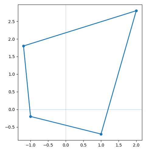

From the last two plots it is easy to extract a few useful properties about f(v):

1. The function is differentiable except for a finite number of points where there are kinks — discontinuities in the first derivative.

2. Each differentiable region corresponds to a vertex of our polygon and when constrained to that region, the function is concave. We will call these regions of the sphere vertex regions. Remember that C = A - B so each vertex region actually corresponds to a pair of vertices, one from A and one from B.

3. From the definition of the support function, the kinks occur when e.g. when
   c₁ • v = c₂ • v, which implies they occur at the point on the sphere satisfying
   (c₁ - c₂) • v = 0. This means v must be perpendicular to the edge of the polygon. In other words the kinks occur at the face normals of C. This is also intuitive, imagine what happens as the support direction sweeps from one vertex to another. In the middle it will be perpendicular to the polygon face and the projection along that direction of both face vertices will be the same.

These properties can be proven using definition of the support function if you want to be rigorous. From calculus, we know that the minimum of f(θ) restricted to a vertex region must occur at the boundary. Then globally the minimum must occur at one of the kink points, this gives us a global solver. We simply evaluate f at all the kink points and pick the minimum value. In this example it is simple to enumerate the kinks because we specified all the vertices which can be used to derive the face normals. In practice we know the vertices of A and B and don’t explicitly construct C. However this is not a problem since supp(A-B, v) = supp(A, v) - supp(B,v) and the kink points of a sum of functions are the union of the kink points from the individual functions. So in practice we would evaluate f at all the normals of A and the normals of B and pick the minimum value. Hopefully you have realized that what we have discovered is the regular separating axis test in 2D. Notice that we didn’t do much geometry, we just used some basic calculus facts. This 2D case is very similar to the 3D case which we will look at next.

General case in 3D

In R² the discontinuities of the support function’s derivative were along lines passing through the origin and the intersection of the lines with the circle were points. In R³ it shouldn’t be a stretch that the discontinuities of the support function are planes passing through the origin and their intersection with the sphere is great circles

If we plot the discontinuities coming from both A and B we get a picture like I showed in the beginning of the article.

In the 3D case our objective function has similar properties to 2D:

1. The vertex region for c_i is bounded by K_i planes. The plane separating two neighboring vertex regions corresponding to c₁ and c₂ is defined by
   (c₁ - c₂) • v = 0.

2. The boundary curve for a vertex region has K_i discontinuities which are located at the face normals. The line of reasoning from 2D can be generalized to 3D. Since the face normals are are intersections of geodesics we have that face normals are orthogonal to the cross product of any two of edges of the face.

3. The minimum of f over a vertex region occurs at the face normals. A similar calculus argument can be used here. The min over the 2D portion occurs at its boundary. The min of the 1D portion occurs at its boundary.

4. The global min can be found by enumerating all face normals (vertex region boundary kinks).

From the last property above we get the separating axis test described by Dirk’s presentation. Namely, iterate over all face normals of the minkowski difference and calculate the projection. The important optimization that Dirk points out is that the new face normals formed by cross products can avoid a full support function evaluation because you know a vertex that lies on the face of the Minkowski difference. We can take this idea further and save the support function evaluation for all face normals (except one) because it should be clear that we can determine neighboring vertex regions for each face normal.

Optimized SAT Test

Here’s the main idea. Traverse the arcs on the sphere using a graph traversal algorithm and as you traverse keep track of the support point for each region. In more detail

1. Pick a point w on one of the arc end points in figure (7) and calculate the vertex region you are in A and -B. I.e. calculate supp(A,w) and supp(-B,w) and keep track of the vertices a, b.

2. Follow the arc and as you move across the sphere keep track of which other arcs you intersect. Every time you hit an arc you enter into a new vertex region.

3. Every intersection or endpoint w you traverse is a face normal and the support function is simply w • (a - b)

Let us consider a concrete example using the diagram below. Denote the face normals by greek letters with α_i, β_i and γ_i corresponding to the face normals of A, -B and the new face normals of A-B respectively.Similarly, the latin alphabet is used to denote the vertex regions of A and -B. That is, if G is the intersection of regions labeled a₁ and b₂ then

10)
    supp(A-B, v) = (a1 - b2) • v 
    for all v in G

Here are the first few iterations of the example

1. Start at α₁ arbitrarily and calculate the the vertex region b₁ using a full evaluation of the support function of B. We know that we are also in a₁ for free. Record
   f(α₁) = α₁ • (a₁ - b₁).

2. Begin traversing the arc from α₁ to α₂ and find that you intersect the arc
   between β₁ and β₃ , the intersection point is γ₄. Record f(γ₄) = γ₄ • (a₁ - b₁).

3. Passing through the plane in the previous step moved you move from region b₁ to region b₂. Keep moving from γ₄ to γ₃ and record f(γ₃) = γ₄ • (a₁ - b₂)

4. Continue on moving from γ₃ to α₂ . Since we intersected another plane defined by the arc between β₂ and β₃ we will update our vertex region to b₃. Record f(α₂) = γ₄ • (a₁ - b₃).

5. Continue this process until all arcs of A have been traversed.

That is pretty much the whole idea. There are a lot of important implementation details like what data structures to use and how to implement arc tracing and intersection tests but this post is already getting too long. If you are curious about the nitty gritty details you can browse the code linked at the beginning and end of the article. In broad strokes these are some of the must haves

Use some variant of a half edge data structure. You need as much topological information you can get. For each vertex I store a flat array of all its connected edges. For each edge I also store the face on each side of the edge.

struct Edge 
{ 
    uint8_t vert0, vert1;
    uint8_t face0, face1; 
};

Sort hull edges topologically by arc connectivity so that during traversal every new arc you traverse you know you have already started or terminated at it.

Ensure your hull builder produces high quality hulls. Like the regular separating axis test, this algorithm is sensitive to the quality of the hull. However I haven’t noticed any numerical issues so far that are any worse than regular SAT.

Conclusion

We’ve covered a different way to look at the Separating Axis Test, not as a purely geometric algorithm, but as an optimization problem on a sphere. By analyzing the properties of the support function, we found its minimum must lie on the "kinks" formed by the intersection of great circles on a Gauss map.

The key insight is that this map is just a graph that we can incrementally traverse. Instead of re-calculating the support function at each node (face normal), we can perform one initial calculation and then traverse the graph, updating the support vertex cheaply as we cross the boundaries (arcs) into new regions. This is essentially the same support function optimization that many physics engines call hill climbing.

If you want to see it in action, I've put together a demo for Visual Studio on Windows where you can compare the two methods and visualize gauss maps. In my testing, this graph-traversal approach is 5-10x faster than the regular SAT for convex hulls with many faces. For hull vs triangle the speed up is ~1.2x due to fewer edge cross products. Additionally, the version of the algorithm implemented in the demo has some numerical problems with triangles. I’m not sure if it’s due to contact generation or collision detection. This problem is completely fixable and I had it working at some point but the branch seems to be lost to the sands of time. Hopefully I can find some time to get it working again.

I discovered this traversal method independently, but as with most problems in computational geometry, it was probably first solved by someone in the 70s. If this algorithm has a name or if you know of any games that use a similar technique, please let me know! I'd love to learn more about its history.

Github repo

Thanks for reading Cairn’s Substack! Subscribe for free to receive new posts and support my work.

GJK is one of the most popular iterative solver but any convex optimization algorithm should work. Iterative methods can also be warm started like GJK using previous solutions. There are a plethora of iterative convex solvers, examples include interior-point methods, gradient descent methods, the ellipsoid method, etc.

However f(v) constrained to the sphere becomes better behaved as origin moves closer to the hull boundary. Below is a cross section of the support function of the unit cube as it is shifted away from the origin. Notice that the support functions starts to look convex away from 0 radians.

A philosophy I learned from Chris Hecker’s great GDC lecture Lemke's Algorithm: The Hammer in Your Math Toolbox