


The Small World of English
The Small World of English
Building a word game forced us to solve a measurement problem: how do you rank 40+ ways to associate any given word down to exactly 17 playable choices? We discovered that combining human-curated thesauri, book cataloging systems, and carefully constrained LLM queries creates a navigable network where 76% of random word pairs connect in ≤7 hops—but only when you deprecate superconnectors and balance multiple ranking signals. The resulting network of 1.5 million English terms reveals that nearly any two common words connect in 6-7 hops through chains of meaningful associations. The mean path length of 6.43 hops held true across a million random word pairs—shorter than we’d guessed, and remarkably stable. 1.5M Headwords 100M Relationships <7 Degrees of Separation for 76% of words
This is consistent with the small-world structure and near-universal connectivity seen in lexical network research on smaller datasets.1,2 The network’s structure makes intuitive semantic navigation possible—players can feel their way from ‘sugar’ to ‘peace’ because the intermediate steps (sweet → harmony) make sense.
sugar → sweet → harmony → peace
The Mathematics of Semantic Distance
English exhibits network effects remarkably similar to social networks—nearly any random pair of words can reach each other in just a few hops through chains of meaningful associations. This “small world” phenomenon was first measured in word co-occurrence networks,3 and persists even after we deprioritize superconnector words that might otherwise dominate many paths.
To probe this, we randomly sampled 1 million word pairs (4 days processing on 32 cores), to get a strong statistical sampling of the connected core of English.
How to connect any random 2 words?
1 0.01% 2 0.15% 3 2.07% 4 9.97% 5 21.58% 6 24.15% 7 18.25% 8 11.18% 9 6.19% 10+ 6.45%Hop Distance Between Words
This bell curve centered at 5-6 hops creates ideal puzzle parameters.
Examples at three distances:
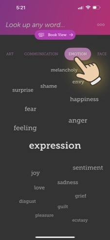
Visual thesaurus mode reveals multiple senses and weighted connections for any word.
Network Construction and Coverage
When we started this project, we tried the obvious approach: combining existing resources like WordNet with early-generation AI tools including LDA topic modeling and static word vectors. WordNet gave us clean synonym sets but lacked the associative richness players expect (“coffee” → “morning” not just “beverage”). LDA found topical clusters but mixed unrelated terms that happened to co-occur. Word vectors collapsed all senses into single points, making “bank” (river) indistinguishable from “bank” (financial). These produced fragmented, overly generic relationships that lacked the nuance our game needed.
We capture 40 associations per term (enough for algorithmic flexibility) and display 17 in our interfaces (what users can reasonably process). This depth provides flexibility for both puzzle generation and reference use.
1,525,522 headwords
We built a semantic network of 1.5 million English terms by casting a wider net than traditional resources. Where academic dictionaries drew sharp boundaries—excluding slang, technical jargon, compound phrases, and proper nouns—we included what people actually say and write. From “ice cream” to “thermodispersion,” from “ghosting” to “Khao-I-Dang.”
This scale would have cost tens of millions to achieve manually. Consider the monumental pre-LLM efforts:
- WordNet (1985-2010) - Princeton’s 25-year project produced 155,000 words in synonym groups. Became the NLP standard despite missing everyday compounds.
- OED (1857-1928, ongoing) - The definitive historical dictionary with 500,000+ entries. Took 70 years and thousands of contributors.
- Webster’s Third (1961) - America’s unabridged dictionary with 476,000 entries. Required 757 editor-years and $3.5 million ($50M+ today).
- Roget’s Thesaurus (1852) - The original meaning-based reference with 15,000 words in 1,000 conceptual categories.
Word counts become arbitrary at this scale. Include every technical term, place name, and slang variant, and the count explodes. Whether we have 1.5 million or 2 million depends entirely on where you draw the line.
Atlas of Connected Meaning
Our inclusion criteria cast a wide net: all terms that volunteer lexicographers at Wiktionary have included (slightly more liberal than typical unabridged dictionaries), plus high-importance Wikipedia topics that are 1-3 words long (measured by PageRank), plus frequently produced compound terms generated by LLMs when analyzing 648,460 Library of Congress book classifications. Compound terms like “local governance” (appearing in 44,507 classifications) and “literary criticism” (19,417) were included, while “wild equids” (5 occurrences) did not.
What kinds of words?
We include all these kinds of words, and to illustrate that there’s no clear redline to include or exclude, here’s a gradation of common and obscure examples of each...
Compounds & Phrases
- “health care” (standard compound)
- “cut the rug” (dated slang for dancing)
- “blow one’s nose” (phrasal verb)
- “hatch, match, and dispatch” (British newspaper jargon)
- “make the welkin ring” (archaic for loud noise)
Slang & Neologisms
- “ghosting” (suddenly ending communication)
- “panda huggers” (political slang)
- “Devil’s buttermilk” (euphemism for alcohol)
- “drungry” (drunk + hungry)
- “brass neck” (British for audacity)
Technical Jargon
- “antibiotics” (medical term)
- “barber-chaired” (logging accident)
- “lead plane” (wildfire aviation)
- “hemicorpectomy” (surgical removal)
- “photonephograph” (kidney imaging)
Species & Taxonomy
- “German shepherd” (dog breed)
- “dwarf sirens” (salamander family)
- “northern raccoons” (regional variant)
- “Angoumois moths” (Sitotroga cerealella)
- “grass crab spider” (specific arachnid)
Historical Language
- “thou” (archaic second person)
- “oftimes” (Middle English)
- “mean’st” (archaic conjugation)
- “crurifragium” (Roman execution)
- “naumachies” (staged naval battles)
Word Variations
- “running” (present participle)
- “rotavates” (tills with rotary blades)
- “masculises” (British spelling)
- “disappoynts” (16-17th century)
- “mattifies” (makes matte)
Acronyms
- “GPS” (Global Positioning System)
- “CICUs” (Coronary Intensive Care Units)
- “HKPF” (Hong Kong Police Force)
- “MIMO-OFDM” (telecom standard)
- “3DTDS” (3-D structural term)
Places & Culture
- “Broadway” (NYC theater district)
- “Harsimus” (Jersey City district)
- “Altai kray” (Russian federal subject)
- “Khao-I-Dang” (refugee camp)
- “ballybethagh” (Irish land measurement)
Rare & Nonce
- “selfie” (once nonce, now standard)
- “greppable” (programmer slang)
- “kiteboating” (water sport)
- “quattrocentists” (1400s scholars)
- “noitamrofni” (information backwards)
Our analysis revealed a fundamental division in the network:
- Reachable terms (56.8%): 870,522 words that appear in the top-40 associations of at least one other word
- Unreachable terms (43.2%): 662,903 words that never appear in any other word’s top-40 list
The unreachable terms include rare compounds (“stewing in one’s own grease”), technical terminology (“thermodispersion”), proper nouns (“Besisahar”), and alternative capitalizations. While these terms can point to other words, no words point back to them strongly enough to rank in any top-40 list. This doesn’t affect puzzles—which start from common words—but reveals an interesting property of the semantic network.
Beyond Traditional Thesauri
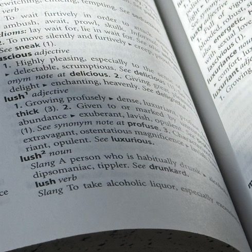
Traditional thesauri focus on synonyms for abstract concepts while excluding concrete objects because they had limited paper pages.
Our visual thesaurus presents up to 8 contextual senses per term, each showing its own 17-word neighborhood. Just as our headword inclusion is necessarily arbitrary, so too is our sense distinction. LLMs identified these senses by querying with various prompts for different meanings and contextual flavors, then merging similar results. We capped it at 8 senses as more became unwieldy in the user interface. Whether “bank” gets 2 senses or 5, whether “coffee” as beverage differs from “coffee” as social ritual—these are judgment calls.
Beyond homographs (words with identical spelling but different meanings, like “bass” for sound versus fish), we capture what we call “contextual flavors” within single senses. ‘Coffee’ connects to ‘café’ (location), ‘beverage’ (category), and ‘espresso’ (variety)—same core meaning, different facets.
Our design philosophy centered on how people think of word associations—pools of related meanings that don’t necessarily align with how dictionaries split formal senses or define when meanings relate. This approach yields an average of 70 semantically connected words per headword across multiple senses, compared to 10-20 in traditional resources. Examples of our relationship types include:
- Similar meanings: house → domicile, lodge
- Category members: house → bungalow, villa
- Functional relationships: horse → saddle, bridle
- Cultural associations: breakfast → coffee, pastries
- Taxonomic connections: quark → boson, fermion
- Domain crossings: quark → Feynman (physics) or quark → cheese (food)
- Thematic groupings: hike, nature, trail
This approach yielded approximately 100 million directed edges connecting our 1.5 million terms.
Try it yourself: What relates to “music”?
Pick any 10 words from the pink box that you think best relate to “music.” There’s no perfect answer—that’s the point.
Great choices! You’ve captured your unique perspective on music.
Multiple Meanings as Network Bridges
English words often carry multiple meanings, creating natural bridges in the network:
Double Meanings
Words with entirely different definitions: “bass” (sound/fish), “tear” (eye/rip)
Related Meanings
Connected definitions: “head” as body part, leadership role, or ship’s bow
Contextual Flavors
“Hiking” as nature experience vs. physical exercise
These multi-sense words create semantic bridges between seemingly unrelated concepts. Words like “ground” can connect earth, coffee, and electrical circuits in a single conceptual leap.
You’d think words with multiple meanings would connect distant parts of the network faster. Turns out they don’t—they just give you more creative ways to navigate the same distance. Our analysis of 100k homograph-containing paths shows they average 6.57 hops versus the 6.43 random baseline. Instead of creating shortcuts, they exist in densely connected regions, offering creative routing options rather than efficiency gains.
So where did we get our data?
Five Data Sources

The Linguabase integrates five complementary knowledge sources into a unified semantic network.
The Linguabase integrates five complementary knowledge sources, each contributing unique strengths to our amalgam scoring system that uses multiple ranking signals—from word frequency and co-occurrence patterns to manually curated relationship scores:
1. In-House Lexicographic Work
Our lexicographer and a team of freelance grad students manually created specialized word lists for 5k varied topics, and associations for polysemous terms and word types like interjections that traditional lexicography treats as “stopwords.” These lists cover many of the most important common terms with multiple meanings.
LLM Generation vs. Recognition
Generation Mode
[safe, clinical terms only]
Recognition Mode
[nuanced connection validated]
2. Mining 125 Years of Library Wisdom
We discovered that LLMs are much better at recognizing valid semantic relationships than generating them from scratch. Ask an LLM “What relates to coffee?” and you’ll get predictable answers: beverage, caffeine, morning. But the Library of Congress classification system revealed that ‘coffee’ appears in 2,542 different book classifications—linking to ‘fair trade certification’ in economic texts, ‘coffee berry borer’ in Hawaiian agriculture books, and ‘import-export tariffs’ in 487 trade policy publications. These connections capture how coffee actually intersects with global commerce, agriculture, and regulation.
Coffee’s 2,542 Library Contexts
Since 1897, LOC catalogers have encoded the intellectual connections between 17 million books, creating what’s essentially a 125-year collaborative knowledge graph built by thousands of subject experts. Each classification represents a moment when a human expert decided “these concepts belong together”—and unlike web text, these decisions were expensive and permanent, made before SEO or engagement metrics existed.
Expert Curation vs. Crowd Wisdom
Web Text
LOC Classifications
We gave an LLM a focused task: generate word lists for each of LOC’s 648,460 classifications. A classification like “Hawaiian coffee trade” triggered specific, expert-like outputs: “kona coffee, arabica beans, coffee tariffs, pacific trade routes, coffee auctions”—far richer than asking generically about coffee. Each classification acted as a pre-engineered prompt that specified exactly which semantic neighborhood we wanted. “Schizophrenia—medical aspects” surfaced “atypical antipsychotic, dopamine antagonist,” while “Schizophrenia—fiction” yielded “asylum writings, trauma memoirs, neurodivergent voices,” capturing the full dimensionality of concepts.
Context Shapes Connections: Schizophrenia
Medical Context
Fiction Context
The real magic came from inverting the index. When we asked “Which classifications contain ‘algorithm’?” we found it appearing not just in computer science but in “aleatory electronic music” (alongside John Cage and stochastic processes), “mathematics in arts” (with fractals and Fibonacci sequences), and “investment mathematics” (with portfolio optimization). The system surfaced connections that require domain expertise: ‘Las Vegas’ linking to ‘Colorado River water rights’ through 12 books about Nevada’s water crisis, or ‘origami’ connecting to ‘shell structures’ and ‘stress analysis’ through engineering texts on deployable structures.
The Double Inversion Process
This approach gave us 3.1 million unique terms weighted by intellectual effort—a monograph on ‘bank equipment’ that mentions ‘pneumatic tubes’ (still used in 15 classifications!) counts more than casual blog mentions. Terms like “cultural heritage” appearing in 53,833 classifications became superconnectors we could appropriately down-rank, while preserving the “boring but essential” connections found in specialized journals like “sewer pipe periodicals” that link urban infrastructure to public health.
Superconnector Term Penalties
The process also revealed what we call the “Montreal effect”—where ‘bagels’ incorrectly associates with ‘Expo 67,’ ‘McGill University,’ and ‘French-speaking’ simply because Montreal is famous for its bagels. Our initial algorithm strengthened these geographic contaminations throughout the data. We resolved these spurious connections through subsequent LLM reviews that could distinguish true semantic relationships (“bagels → boiled dough → chewy texture”) from coincidental geographic co-occurrence (“bagels → Montreal Canadiens”).
The Montreal Effect: Geographic Contamination
❌ Geographic Co-occurrence
✓ True Semantic Relations
3. Human-Curated Resources
Over 70 existing references contributed—dictionaries, thesauri, and encyclopedias from Wiktionary and WordNet to specialized resources like NASA’s thesaurus and the National Library of Medicine’s UMLS. Relationships appearing across multiple sources received higher weights.
General Sources
- Wiktionary
- WordNet, ConceptNet, FrameNet
- Roget’s Thesaurus
- SWOW-EN18
Specialized Sources
- Getty Art & Architecture
- NASA Thesaurus
- UMLS Metathesaurus
- AGROVOC Thesaurus
4. Pre-LLM Topic Extraction
Before the rise of modern LLMs, we applied Latent Dirichlet Allocation (LDA) in 2013-2014 to discover eight context clusters for every headword in an in-house corpus of notable literary works. The algorithm scans large text collections and groups words that appear in similar contexts. Running it took 200,000 super-computer hours on the NSF’s Extreme Science and Engineering Discovery Environment (XSEDE)—decades on a single machine. Results were noisy: a delightful mix of intuitive associations and oddities (often caused by treating compound terms as separate words). Still, the run surfaced relationships that pure frequency analysis and today’s LLMs miss.
We skipped early word-embedding vectors—numeric coordinates that place context-similar words near one another but merge all senses into one point—because, as games like Semantle show, their distances rarely match human intuition. We also evaluated word embeddings but their single-vector-per-word approach couldn’t handle our need for multiple senses—a fundamental limitation that various researchers tried to patch.5
5. Large Language Model Enhancement
Starting in 2023, frontier models finally provided the semantic understanding we needed—they could distinguish “bank” (river) from “bank” (money) and generate contextually appropriate associations for each. These models could handle:
- Everyday compound terms (“apple pie”, “department store”)
- Morphological variations across parts of speech
- Contextual dimensions of common words
- Capitalization distinctions (“China” vs. “china”)
Still, left to their own devices, LLMs are banal and formulaic, wallowing in cliche, latching onto what they think prompts intend. We ran over 80 million API calls (~$200k in Azure API costs, with minor xAi costs) across dozens of workflows to combat this tendency. Beyond the LOC classifications, we applied focused-prompt strategies across our entire corpus: extracting distinct senses for each headword, generating contextual word lists per sense, prompting for cultural variations and regional differences. Each workflow fed into the next—outputs from sense detection became inputs for association generation, which informed cultural expansion passes. The key was always the same: constrained, specific prompts yielded far better results than open-ended queries.
Even with careful prompting, the Montreal effect persisted. Geographic contamination appeared throughout: ‘Broadway’ linked to ‘taxis’ through New York; ‘grits’ to ‘jazz’ through the American South. We resolved these spurious connections through iterative LLM reviews that learned to distinguish true semantic relationships from coincidental geographic co-occurrence. This research and computational scale was made possible by $295k NSF SBIR seed funding (#2329817) and $150k Microsoft Azure compute resources.
Understanding Our Biases
Every semantic network encodes particular worldviews about which words relate to each other and how strongly they connect. Here are six key sources of bias that shape our network’s rankings and inclusions:
| Editorial Choices | AI Training Data |
|---|---|
| Our lexicographer and team manually crafted relationships for common polysemous terms, inevitably encoding their linguistic backgrounds, cultural contexts, and conceptual frameworks about how meaning connects. Examples: “market” → includes “variety” and “retail,” omits “souk,” “bazaar” • “breakfast” → includes “cereal,” “toast,” omits “congee,” “idli” • “music” → includes “jazz,” “consonance,” omits “gamelan,” “qawwali” | GPT-4o’s training data shapes its semantic associations, while its guardrails suppress certain connections. We supplemented with Grok-3 specifically for vulgar and offensive terms that GPT-4o wouldn’t adequately cover. Examples: “sex” → clinical terms favored over colloquial language • “death” → euphemisms like “passing” prioritized over direct terms like “corpse,” “decay” |
| Superconnector Deprecation | Prompting Cascades |
| No matter how a large thesaurus is constructed, certain terms seem to be ubiquitous. This is partially author bias, partially natural language structure, and worse with repetitive LLMs. We down-rank ubiquitous words like “heritage” and “surname”—a low-key version of inverse-frequency normalization. Our graduated penalty system scores 59,112 terms with an inverse document frequency (IDF) variant that down-ranks common terms (1-18). Surprisingly, penalty correlates with conceptual breadth, not raw frequency: “heritage” (penalty 18) appears only 201 times, while “tourism” (penalty 14) appears 8,520 times. Examples: At one processing stage, 2 words get maximum penalty (18): “surname” and “heritage” • 46,445 words get minimal penalty (1) • “heritage” can connect to almost anything cultural, historical, or traditional | Our multi-pass LLM workflow (listing senses → expanding culturally → reprocessing) introduces systematic preferences that affect both what gets included and how highly it ranks. Examples: Geographic diversity emphasized, so “dance” includes global forms equally • Cultural foods given comparable rankings to Western staples |
| Frequency ≠ Importance | Morphological and Similarity Filters |
| Frequency is a useful but flawed proxy for word importance. It captures actual usage but creates artifacts: ‘pandas’ outranking ‘panda,’ ‘cheesecake’ outranking ‘cheesecakes,’ literary corpora overweighting ‘thee,’ technical terms underrepresented. Different corpora (books vs. screenplays) produce subtly different hierarchies, and none capture a word’s actual utility for learners or gameplay. Examples: “pandas” plural outranks “panda” • “thee” elevated by Shakespeare • “cheesecake” singular is more common than “cheesecakes” • Literary bias from Google N-grams. | Nobody wants word clouds full of plurals and variants. Our filter pushes ‘baguettes’ down 30 positions if ‘baguette’ already appears, ‘rolls’ down 23 if ‘roll’ exists (>90% string similarity gets +12 penalty, plural/singular differences +17, reordered compounds +17). Length penalties also apply progressively. Examples: In “bagels” - “baguette” drops 30 positions because “baguettes” appears earlier • “roll” drops 23 positions when “rolls” is present • Singular forms consistently cascade downward when plurals exist |
These biases shape which connections appear, how strongly they’re weighted, and where they rank in each word cloud. We’ve made deliberate choices to create a semantic network optimized for engaging gameplay—favoring conceptual diversity over raw frequency, meaningful connections over statistical noise. The Linguabase represents one coherent mapping of English’s semantic landscape, designed to reveal the surprising paths that connect all words.
How Network Properties Enable Gameplay
The mathematical properties of our semantic network create natural game parameters:
We tested various difficulties and settled on 3-7 hops. Below 3 felt trivial; above 7, players gave up. The 3-hop puzzles naturally yield 27 solutions when we maintain 3 strong choices per step.
For virtually any common word selected as a puzzle origin, there are ~370 million outward paths within 7 hops (about 10% less than the 17&sup7;=410 million theoretical maximum due to natural graph loops). Within those paths, only 200k-1 million reach the target—a random success rate of 0.05-0.27%. Players succeed at much higher rates because they navigate semantically rather than randomly. Our puzzles are engineered to ensure at least 3 good choices per hop, creating exactly 27 optimal three-hop “Genius” solutions (3³ paths).
Theoretical Maximum (if no word overlap)
3 hops: 17³ = 4,913 paths
4 hops: 17&sup4; = 83,521 paths
5 hops: 17&sup5; = 1,419,857 paths
6 hops: 17&sup6; = 24,137,569 paths
7 hops: 17&sup7; = 410,338,673 paths
Measured Reality (with semantic overlap)
Total paths: ~370 million (90% of theoretical)
Winning paths: 200k-1 million
Beyond game limit: ~94% require 8+ hops
Curious how we transformed this linguistic database into a daily word game? Read Making the Game to discover how we found the perfect game mechanic and balanced the difficulty.
Further
Explorations
References
By Michael Douma, Greg Ligierko, Li Mei, and Orin Hargraves
A product of Institute for Dynamic Educational Advancement (IDEA.org)
What's Your Reaction?
 Like
0
Like
0
 Dislike
0
Dislike
0
 Love
0
Love
0
 Funny
0
Funny
0
 Angry
0
Angry
0
 Sad
0
Sad
0
 Wow
0
Wow
0