Convolutions, Polynomials and Flipped Kernels

Multiplying polynomials

Suppose we want to multiply one polynomial by another:

This is basic middle-school math - we start by cross-multiplying:

And then collect all the terms together by adding up the coefficients:

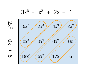
Let's look at a slightly different way to achieve the same result. Instead of cross multiplying all terms and then adding up, we'll focus on what terms appear in the output, and for each such term - what its coefficients are going to be. This is easy to demonstrate with a table, where we lay out one polynomial horizontally and the other vertically. Note that we have to be explicit about the zero coefficient of x in the second polynomial:

The diagonals that add up to each term in the output are highlighted. For example, to get the coefficient of

• The coefficient of
• The coefficient of in the second polynomial
• The coefficient of in the first polynomial, multiplied by the coefficients of

(if the second polynomial had a

For what follows, let's move to a somewhat more abstract representation: a polynomial P can be represented as a sum of coefficients x

Suppose we have two polynomials, P and R. When we multiply them together, the resulting polynomial is S. Based on our insight from the table diagonals above, we can say that for each k:

And then the entire polynomial S is:

It's important to understand this formulation, since it's key to this post. Let's use our example polynomials to see how it works. First, we represent the two polynomials as sequences of coefficients (starting with 0, so the coefficient of the constant is first, and the coefficient of the highest power is last):

In this notation, P, etc. To calculate the coefficient of

Expanding the sum for all the non-zero coefficients of P:

Similarly, we'll find that

There's a nice graphical approach to multiply polynomials using this idea of pairing up sums for each term in the output:

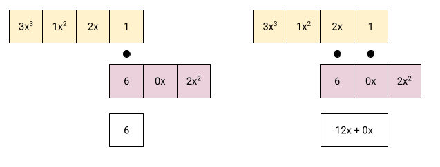
We start with the diagram on the left: one of the polynomials remains in its original form, while the other is flipped around (constant term first, highest power term last). We line up the polynomials vertically, and multiply the corresponding coefficients: the constant coefficient of the output is just the constant coefficient of the first polynomial times the constant coefficient of the second polynomial.

The diagram on the right shows the next step: the second polynomial is shifted left by one term and lined up vertically again. The corresponding coefficients are multiplied, and then the results are added to obtain the coefficient of x in the output polynomial.

We continue the process by shifting the lower polynomial left:

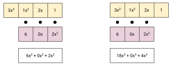
Calculating the coefficients of

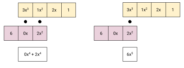
Now we have all the coefficients of the output. Take a moment to convince yourself that this approach is equivalent to the summation shown just before it, and also to the "diagonals in a table" approach shown further up. They all calculate the same thing

Hopefully it should be clear why the second polynomial is "flipped" to perform this procedure. This all comes down to which input terms pair up to calculate each output term. As seen above:

While the index i moves in one direction (from the low power terms to the high power terms) in P, the index k-i moves in the opposite direction in R.

If this procedure reminds you of computing a convolution between two arrays, that's because it's exactly that!

Signals, systems and convolutions

The theory of signals and systems is a large topic (typically taught for one or two semesters in undergraduate engineering degrees), but here I want to focus on just one aspect of it which I find really elegant.

Let's define discrete signals and systems first, restricting ourselves to 1D (similar ideas apply in higher dimensions):

Discrete signal: An ordered sequence of numbers

Discrete system: A function mapping input signals

Here's an example signal:

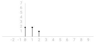
This is a finite signal. All values not explicitly shown in the chart are assumed to be 0 (e.g.

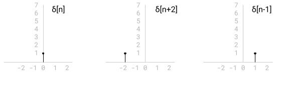
A very important signal is the discrete impulse:

In graphical form, here's n, correspondingly. Take a moment to double check why this works.

The impulse is useful because we can decompose any discrete signal into a sequence of scaled and shifted impulses. Our example signal has three non-zero values at indices 0, 1 and 2; we can represent it as follows:

More generally, a signal

(for all k where

In the study of signals and systems, linear and time-invariant (LTI) systems are particularly important.

Linear: suppose a and b are constants.

Time-invariant: if we delay the input signal by some constant:

LTI systems are important because of the decomposition of a signal into impulses discussed above. Suppose we want to characterize a system: what it does to an arbitrary signal. For an LTI system, all we need to describe is its response to an impulse!

If the response of our system to

• Its response to c, because the system is linear.
• Its response to k, because the system is time-invariant.

We'll combine these and use linearity again (note that in the following

Is:

This operation is called the convolution between sequences

Let's work through an example. Suppose we have an LTI system with the following response to an impulse:

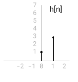
The response has

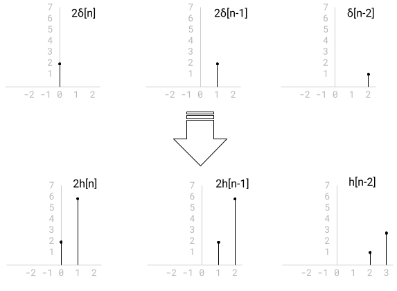
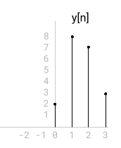
The top row shows the input signal decomposed into scaled and shifted impulses; the bottom row is the corresponding system response to each input. If we carefully add up the responses for each n, we'll get the system response

Now, let's calculate the same output, but this time using the convolution sum. First, we'll represent the signal x and the impulse response h as sequences (just like we did with polynomials), with

The convolution sum is:

Recall that k ranges over all the non-zero elements in x. Let's calculate each element of h is nonzero only for indices 0 and 1):

All subsequent values of y are zero because k only ranges up to 2 and

If you look carefully at this calculation, you'll notice that h is "flipped" in relation to x, just like with the polynomials:

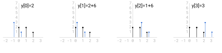
• We start with
• In subsequent steps, y is computed by adding up the element-wise products of the lined up x and h.

Just like with polynomials k), while the other decreases (n-k).

Properties of convolution

The convolution operation has many useful algebraic properties: linearity, associativity, commutativity, distributivity, etc.

The commutative property means that when computing convolutions graphically, it doesn't matter which of the signals is "flipped", because:

And therefore:

But the most important property of the convolution is how it behaves in the frequency domain. If we denote f, then the convolution theorem states:

The Fourier transform of a convolution is equal to simple multiplication between the Fourier transforms of its operands. This fact - along with advanced algorithms like FFT - make it possible to implement convolutions very efficiently.

This is a deep and fascinating topic, but we'll leave it as a story for another day.