


Compiling a neural net to C for a speedup

Compiling a Neural Net to C for a 1,744× speedup
2025-05-27 · About 25 minutes long
tl;dr: I trained a neural network (NN), with logic gates in the place of activation functions, to learn a 3×3 kernel function for Conway’s Game of Life. I wanted to see if I could speed up inference by extracting the learned logic circuit from the NN. So, I wrote some code to extract and compile the extracted logic circuit to bit-parallel C (with some optimizations to remove gates that don’t contribute to the output). I benchmarked the original NN against the extracted 300-line single-threaded C program.; compiling the NN to C resulted in a 1,744× speedup! Crazy, right? Here’s the repo: ~354 lines of Python/JAX, ~331 lines of C, if you want to reproduce it and/or mess around.
The longer story
While plumbing the intertubes (as one does), I came across this fun publication by the Self Organising Systems group at Google, about Differentiable Logic Cellular Automata. This research caught my attention (I mean, who doesn’t love a pretty picture), and as I read it, I realized the whole idea wouldn’t be too hard to replicate. (Which is crazy, because this is crazy. I mean, the authors cite creating computronium as a source of inspiration. Awesome!)
To break things down a little bit: Differentiable Logic Cellular Automata is a quite a mouthful, I know, but the idea is the straightforward composition of two existing ideas:
-
Cellular Automata (CA) are grids of cells, where each cell changes over time according to some local rule. The most famous cellular automata are Conway’s Game of Life and perhaps Rule 110. We call this local update rule a kernel, a function that looks at the local neighborhood around a cell to calculate the cell’s next state. By applying the kernel to each cell in our grid, we step the cellular automata forward through time. Simple rules can give rise to strikingly complex behaviour. Neural Cellular Automata (NCA) are a variant of CA that replace the kernel function with a neural network. NCA can be trained to learn known kernels (what I do), or more generally, to learn kernels that give rise to a specified target behavior.
-
Deep Differentiable Logic Gate Networks (DLGNs) are like neural networks, with two key differences. First, the weights are fixed, and set to 0 or 1; each neuron has exactly two inputs (one left, one right) We call these weights wires. Since wires are fixed, we learn the activation function. In this case, our activation function is a weighted linear combination of a set of 16 logic gates, applied to the two inputs. Essentially, we learn which logic gate should be used for each node in a fixed circuit. (If you’re a little lost, don’t worry, later, I’ll go into more detail to describe what this looks like in practice.)
After reading the original publication, I wanted to play with a few different experiments. To start, I wanted to replicate the research without looking at it too closely, to give room for creative misinterpretation, to understand what decisions were important. I also wanted to mess around with whatever the result of that was, until something interesting fell out. Consider this to be something of a pilot episode: there is a lot I still would like to experiment with. (Like fluid simulation! We could find a circuit for the kernel rule for Reintegration Tracking. Wouldn’t that be neat?)
I tried something new for the first time, which was to keep a journal during development. I have no idea why I’ve never done this before, because it made recording training runs, figuring out what to debug, tracking next steps, and scoping changes so much easier. (Not to mention writing this write-up!) This project took three days (well, four five if you count this write-up), and it’s cool to see how much progress I made each day.
Conway’s what? A quick recap
Conway’s Game of Life is a Cellular Automata that takes place on a 2D grid of square cells. Each cell has 8 neighbors. At each step, looking at this 3×3 neighborhood, we decide whether each cell is alive or dead, according to two rules:
- If the cell has exactly 3 live neighbors, it is alive.
- If the cell has exactly 2 live neighbors, and is alive, it remains alive.
I guess there’s a harsh third rule which is, “if the cell is dead, it stays dead”. You may already begin to see how this could be written as a logic circuit. Here’s one way: given an array, inputs, with 9 cells where 0 is dead, 1 is alive, we can write:
n = sum(inputs) - alive # neighbors excluding center
alive_next = (n == 3) or ((n == 2) and alive)
The hard part, you might glean, would be coming up with a compact circuit for counting n, the number of neighbors. That’s what we’re up against: given a 9-bit input, we’re going to try to learn a circuit of logic gates whose output matches the 1-bit alive_next output, end-to-end.
N.B. You should try coming up with a circuit yourself, by hand! I did, it’s not too crazy. Here’s a hint: A cell has 8 neighbors. You can count how many cells are alive for any pair of inputs:
xorfor 1,andfor 2. Can you use two pairs to count 4? What about 8? Once you can determine whether the neighborhood count is 2 or 3, the rest is fairly straightforward. How many logic gates did you use? How deep is your circuit?
In the beginning was JAX
Now, I suppose I’ll show my age by saying that my knowledge of ML frameworks is stuck around 2017, with old Keras (never change, Sequential) and TensorFlow (before 2.0). I used to mess around with GANs (StyleGAN <3) and I even implemented RND on top of PPO at some point! So I have a good intuition of the basics. Much has been lost to the sands of time, aside from a handful of random projects shotgunned across GitHub. Sigh.
Well, as Oogway would say, “Yesterday is history, tomorrow is a mystery, but today… is a gift. That is why it is called the present.” There is no better day than today to get back on your A-game.
JAX is a machine learning framework for Python. I think of it as numpy on steroids. JAX has an API-compatible implementation of numpy living at jax.jnp: you can do all the fun matrix stuff (like multiplication!) and you get a couple things for free:
- grad will compute the gradient of any non-sadistic function. It does this using automatic reverse-mode differentiation, but you can get as fancy as you’d like.
- vmap will automatically parallelize and vectorize computations that can be run in parallel. For example, I use vmap to batch training in my implementation.
- jit will just-in-time compile all of the above, and can produce code that runs on the GPU. Compiling Python at the library level using decorators is crazy!
JAX has an ecosystem of libraries that mix and match these operations to build more powerful primitives. Optax, for example, implements common optimization strategies, like adamw, on top of jax.grad. Flax, is a NN library built on top of JAX. (Tbh, flax is a little confusing: there’s nn (deprecated), linen, nnx. Everyone uses linen but the flax devs want people to use nnx it seems).
N.B. One other thing I like about JAX is that randomness is reproducible. All functions that generate non-deterministic output take a RNG key, and keys can be split into subkeys. The root key is generated when you set the seed; everything else derives from the root key. This means if you run a program twice, you’ll have the same initialization, same training samples, same convergence. It makes debugging a lot easier, because you can reproduce e.g. a blow-up during training with some patience.
Continuous relaxation
To learn a circuit, we need some way to translate the hard, discrete language of logic into the smooth, continuous language of gradients. (Gradients, now those are something an optimizer can get a handle on!)
A logic gate, like and(a, b), is a function of two inputs; we can arrange them into a table like so:
| 0 | 1 | |
| 0 | 0 | 0 |
| 1 | 0 | 1 |
Here, inputs are defined to be exactly 0 or 1. What if the inputs vary between 0.0 and 1.0; is there a continuous function of two inputs f(a, b) that behaves like and(a, b) at the boundary? Well, yes, f(a, b) = a * b fits the bill. We can say that a * b a continuous relaxation of and(a, b). There are 16 fundamental logical functions of two inputs; here they all are, along with a continuous relaxation for each:
| gate | relaxation | gate | relaxation |
|---|---|---|---|
false | 0. | true | 1. |
and | a*b | nand | 1. - a*b |
a&~b | a - a*b | b/~a | 1. - a + a*b |
a | a | not a | 1. - a |
b&~a | b - a*b | a/~b | 1. - b + a*b |
b | b | not b | 1. - b |
xor | a+b - 2.*a*b | xnor | 1. - (a+b - 2.*a*b) |
or | a+b - a*b | nor | 1. - (a+b - a*b) |

This is great! (It’s fun to try to derive continuous relaxations yourself.) With this groundwork in place, we could create a “learnable logic gate” of sorts by taking a weighted sum of each relaxation. In JAX, using jnp:
jnp.sum(gate_weight * gate_all(left, right)) # axis=0
Here, gate_all returns a vector where each entry is the result of one of the functions above. If we want to make sure that the gate weights stay in a reasonable range, we can apply a softmax to the learned vector w, which squashes each gate weight to be between 0.0 and 1.0:
gate_weight = jnp.exp(w) / jnp.sum(jnp.exp(w)) # axis=0, keepdims=True
We can train a network to learn these gate weights. Once we have a trained network, can replace the softmax with an argmax (taking the gate with the highest weight). This gives us a circuit with a hard 0 or 1 as an output; a discrete logic gate is also much cheaper to compute. (It’s almost as if computers are full of them!)
Hardness zero
Well, we have our continuous relaxations and we have a NN. Let’s just put them together, replace relu with gate, and call it a day? Not so fast.
Machine learning papers almost make research look effortless, as though NNs magically converge when enough data is forced through their weights. This could not be further from the truth: there are so many failure modes; so many experiments that have to be run to guess the right hyperparameters; training a NN requires a weird combination of patience (giving the model enough time to converge) and urgency (stopping runs early when something is wrong). It’s fun, but it can also be frustrating, yet somehow addicting.
I could skip over the two days of elbow grease it took to get this working. However, differentiable logic gate networks train a little differently than your standard dense relu network, and there were a couple things, like how you initialize DLGNs, that surprised me.
Wiring
At the start of this project, I wanted to see if I could learn the wires in addition to the gates. I still think it’s possible, but it’s something I had to abandon to get the model to converge.
I started this project by writing a simple dense NN with relu activation and standard SGD, just to see if things were working. They were, and my small model converged very quickly!
In traditional NNs, it’s commonly-accepted wisdom that you should initialize the wire weight matrices according to a tight normal distribution centered around zero. This is what I did for the relu network above, and it worked like a charm!
I switched from relu to gate by adding two weight matrices per layer, one for the right gate input, the other for the left. After this switch, however, try as I might, the model would not converge. I also started to worry about whether having negative wire weights would make it hard to extract the logical circuit after training. So, I thought some more, and decided to initialize wire weights uniformly between 0 and 1. This performed even worse!
Thinking some more, I had an epiphany: “well, since the goal is to learn a wiring, we should softmax the wires in the same way we softmax the gates!” In desperation, I implemented a row-wise softmax over wire weights initialized uniformly… this also went about as well as you would expect. (Poorly.)
At this point I realized: maybe a fixed 1 or 0 wiring is not just a random choice, but highly essential! Wouldn’t a fixed wiring let the gradients propagate all the way to the gates at the input end of the network, so the gates at the output end of the network could begin to converge? I began to look at how wiring was implemented in the paper; I decided to abandon my learned-wiring dreams for the time being.
In hindsight, it’s obvious that how you wire a network determines how information flows through it, so it’s important that the wiring is good, especially if the wiring is fixed. I don’t know why it took me so long to realize this.
After I refactored everything to use fixed wiring, I first I tried completely random wiring. This did a lot better than any of the previous approaches, but was still nowhere near the publication. After careful inspection, I realized that with this approach, you risk not wiring gates, or wiring two gates the same way, losing information as it flows through the network.
My next thought was to wire the network like a tree. We had descending power-of-two layers: 64, 32, 16, 8, 4, 2, 1; what if each layer was connected to the corresponding two cells in the layer before it? This way there is total information flow. Tree wiring worked like a charm, and it was at this point that I started to have hope.
I read the publication more closely, and at this point I looked at the colab notebook. The wiring technique used is interesting: it guarantees we get unique pairs, like tree wiring, but we also shuffle the branches between layers to allow for some cross-pollination. The algorithm looks something like this:
def wire_rand_unique(key, m, n):
    key_rand, key_perm = random.split(key)
    evens   = [(0, 1), (2, 3), ...]
    odds    = [(1, 2), (3, 4), ...]
    padding = rand_pairs_pad(key_rand, m, n)
    pairs   = jnp.array([*evens, *odds, *padding])
    perm    = random.permutation(key_perm, pairs)
    return wire_from_pairs(perm.T, m, n)
(Note that as long as n ≤ m ≤ 2×n, there will be total network connection with no random padding.)
With the wiring from the publication implemented, the model was within spitting distance of fully converging! That’s when one last revelation shook me to my bones.
Initialize gates to pass through
The biggest surprise was the way you’re supposed to initialize the gate weights of a differentiable logic gate network; of course, it now makes 100% sense in hindsight.
Here’s the big idea: we want the gradients to reach the input of the network, but if we initialize gate weights uniformly, or even randomly, we’ll get a flat activation function. Flat activation functions kill all gradients, period. I realized this was happening when I wrote code to visualize each layer in the network, and watched it change over time:
# [...]
layer 3 (16, 8)
▄ ▄ ▄ ▄ ▄ ▄ ▄ ▁ ▄ ▄ ▄ ▁ ▄ ▁ ▁ ▁
▄ ▄ ▄ ▄ ▄ ▄ ▄ ▁ ▄ ▄ ▄ ▁ ▄ ▁ ▁ ▁
▁ ▁ ▁ ▁ ▁ ▁ ▁ ▁ ▁ ▁ ▁ ▁ ▁ ▁ ▁ █
▁ ▁ ▁ ▄ ▁ ▄ ▄ ▄ ▁ ▄ ▄ ▄ ▄ ▄ ▄ ▄
▁ ▁ ▁ ▁ ▁ ▁ ▄ ▁ ▁ ▁ ▁ ▁ ▁ ▁ ▁ ▁
▄ ▄ ▄ ▁ ▄ ▁ ▁ ▁ ▄ ▁ ▁ ▁ ▁ ▁ ▁ ▁
▁ ▁ ▁ ▁ ▁ ▁ ▁ ▁ ▁ ▁ ▁ ▁ ▁ ▁ ▁ █
▁ ▁ ▁ ▁ ▁ ▁ ▁ ▁ █ ▁ ▁ ▁ ▁ ▁ ▁ ▁
layer  4 (16, 4)
▁ ▁ ▁ ▁ ▁ █ ▁ ▁ ▁ ▁ ▁ ▁ ▁ ▁ ▁ ▁
▄ ▄ ▄ ▁ ▄ ▁ ▁ ▁ ▄ ▁ ▁ ▁ ▁ ▁ ▁ ▁
▁ ▁ ▁ ▁ ▁ ▁ ▁ █ ▁ ▁ ▁ ▁ ▁ ▁ ▁ ▄
▁ ▁ ▁ ▁ ▁ ▁ ▁ ▁ ▁ ▁ █ ▁ ▁ ▁ ▁ ▁
layer 5 (16, 2)
▁ ▁ ▁ ▁ ▄ ▁ █ ▁ ▁ ▁ ▁ ▁ ▄ ▁ ▄ ▁
▁ ▁ ▁ ▁ ▁ ▁ ▁ ▁ ▁ ▁ █ ▁ ▁ ▁ ▁ ▁
layer 6 (16, 1)
▁ ▁ █ ▁ ▁ ▁ ▁ ▁ ▁ ▁ ▁ ▁ ▁ ▁ ▁ ▁
F & . A . B X / / X B . A . & F
                ~~~~~~~~~~~~~~~
# gate order
| FALSE | AND  | A&!B  | A    |
| B&!A  | B    | XOR   | OR   |
| NOR   | XNOR | NOT B | A/!B |
| NOT A | B/!A | NAND  | TRUE |
With dead gradients, I’d see the output gate converge, then the one before it, and so on until the gradients reached the input, at which point the later gates were so fixed in their ways that they were impossible to change, even as better earlier gate weights were discovered. Obviously, the performance of the network plateaus shortly thereafter.
I didn’t see an obvious way around this problem, so I started to wonder if there was some weird trick to get around the problem… and there was. So I read the code.
Of all the gates, these two stand out:
| gate | relaxation | explanation |
|---|---|---|
a | a | Forward a, drop b. |
b | b | Forward b, drop a. |
These pass-through gates do no mixing, and will propagate gradients straight along their wires, all the way to the input! This is critical! And in retrospect, I had missed a seemingly-innocuous line:
To facilitate training stability, the initial distribution of gates is biased toward the pass-through gate.
Of course it is biased! There’s no way to train the network otherwise! So I made a simple one-line change, and, like that, test_loss_hard: 0. Perfect convergence:
Epoch (3001/3001) in 0.0031 s/epoch
[ 0.999 0.999 0.00173 0.000287 0.000537 ] [1. 1. 0. 0. 0.] [1. 1. 0. 0. 0.]
train_loss: 0.000738; test_loss: 9.91e-05; test_loss_hard: 0
At long last, it all fits together.
Hyperfrustration
What frustrates me is that, after correctly implementing the architecture from the publication, the main issues preventing convergence were seemingly arbitrary hyperparameter choices. In my journal I wrote:
The model training code was good, as was the gate implementation. So what was wrong?
- The model was the wrong size (way too small).
- The model was initialized the wrong way (randomly, instead of with gate passthrough).
- The model did not have clipping in the optimizer, which seems like a rather arbitrary, hacky hyperparameter choice.
Hyperparameters suck! I hate that I was pulling my hair out over why I wasn’t getting the same results when all that was different were the hyperparameters at play.
I wonder how many research breakthroughs are possible but just sitting in hyperparameters beyond reach?
Rather existential, I suppose. There are lots of other things I tried that didn’t work. Earlier, I tried to learn the wiring in addition to gates, but the network wouldn’t converge. I thought it was because the network was too complex, but now I’m convinced it’s because it was too small and initialized incorrectly. There is so much more I would like to try.
N.B. All this wiring got me thinking about gaussian splatting of all things. You see, I was recently reading a paper about when to split gaussian splats; the rough idea is to split whenever the optimizer encounters a saddle with respect to any one splat. While watching underparameterized gate networks train, I would see them get stuck between a handful of gates on a given layer, and not converge further. I wonder if it would be possible to build a circuit network that grows over time, splitting gate saddles when loss stops going down? I suppose that’s what inspired the splat paper, so we’ve come full circle.
Extracting the circuit
At this point we have learned a perfect binary circuit that looks at a 3×3 cell neighborhood and computes the game of life kernel. Only one problem: This circuit is stuck as a pile of floating point numbers, tangled up in the vast sea of gate weights and wires. How will we ever get it out?
By compiling it to C.
This isn’t as hard as it sounds. All we have to do is traverse the network, layer by layer. We use our old friend argmax to figure out which wires and gate to use for each gate in the circuit.
At this point, we have a massive network. However, only a tiny fraction of the gates are used! (Most gates are still pass-through.) So I implemented two optimizations to clean up the circuit:
Dead code elimination gets rid of all gates that do not contribute to the output. We’re not doing anything fancy here, like testing for truisms; just doing the simple thing and taking the transitive closure of all dependencies, starting from the root output, going backwards:
def ext_elim(instrs, root):
    out = []
    req = set([root])
    for instr in instrs[::-1]:
        (o, idx, l, r) = instr
        if o in req:
            req = ext_add_deps(req, idx, l, r)
            out.append(instr)
    return list(out[::-1])
Copy propagation lets us get rid of all those pesky useless pass-through gates by forwarding their output to all downstream gates. This time we go forward, and keep track of what to rename pass-through gates.
def ext_copy_prop(instrs, root):
    out = []
    rename = dict()
    for instr in instrs:
        (o, idx, l, r) = instr
        if l in rename: l = rename[l]
        if r in rename: r = rename[r]
        if o == root: out.append((o, idx, l, r))
        elif idx == 3: rename[o] = l
        elif idx == 5: rename[o] = r
        else: out.append((o, idx, l, r))
    return out
(Index 3 and 5 are the indices of the pass-through gates.)
After this, we do a simple rename for all gates (since we’ve decimated the number of gates in use), and emit C. This is just a big switch-case:
def ext_gate_name(idx, l, r):
    names = [
        lambda a, b: "0",
        lambda a, b: f"{a} & {b}",
        lambda a, b: f"{a} & ~{b}",
        # ...
        lambda a, b: f"~({a} & {b})",
        lambda a, b: "~0",
    ]
    return names[idx](l, r)
After formatting, we get a long list of instructions that looks like this:
cell conway(cell in[9]) {
    // ... 157 lines hidden
    cell hh = hc ^ gs;
    cell hi = hb & ~gy;
    cell hj = hh & hi;
    cell hk = hg & cy;
    cell out = hj | hk;
    return out;
}
And like that, all your floats are belong to us. Here’s the final tally for each basic logical operation used in the circuit. (Note that some gates, e.g. nand, are composed of multiple operations):
| Gate | Count |
|---|---|
and | 69 |
or | 68 |
xor | 17 |
not | 16 |
| total | 170 |
Nice. I don’t know why, but it’s satisfying to see a pretty even split between and and or, as with xor and not. I wonder what the distribution looks like in real-world code. (I thought I never used xor, but then I realized that != is really just xor in disguise.)
Bit-crunching C
I pulled a sneaky little trick. I don’t know if you noticed. Here’s a hint:
typedef uint64_t cell;
That’s right: a cell is not one grid cell, but 64! When we calculate cell conway(cell in[9]);, we are, through bit-parallelism, computing the rule on 64 cells at once!
We compile to C and produce a function containing the circuit, conway, but we need a runtime to saturate it. I took a compilers class this semester (6.1100), so I have been writing a lot of Unnamed Subset of C this semester. With C on the mind, I wrote a little runtime. Here’s how it works.
First, I define a board as a collection of cells:
typedef struct {
    cell* cells;
    size_t cells_len;
    size_t width;
    size_t height;
} board_t;
Each cell is just a horizontal slab, 64 bits wide. I’m lazy here, so I require width be a multiple of 64. We initialize this board with random state using an xorshift prng I am currently lending from Wikipedia:
// https://en.wikipedia.org/wiki/Xorshift
// constant is frac(golden_ratio) * 2**64
// global state bad cry me a river
uint64_t rand_state = 0x9e3779b97f4a7c55;

uint64_t rand_uint64_t() {
    uint64_t x = rand_state;
    x ^= x << 13;
    x ^= x >> 7;
    x ^= x << 17;
    rand_state = x;
    return x;
}
On to the meat and potatoes. The function conway requires a list of 9 cells. The neighbors directly above and below are easy: we just index forward or back a row in cells. The side-by-side neighbors are a bit harder. Luckily, we can just bitshift to the left and right to create two new boards. This works as long as we’re careful to catch all bits that might fall into the bitbucket when we shift:
void board_step_scratch_mut(
    board_t *board,
    board_t *scratch_left,
    board_t *scratch_right, // syntax highlighting breaks without a comma here, sigh
) {
    // 5: dense loops and bitshifts,
    // 7: no beauty I can present.
    // 5: click the link above.
}
I guess a better illustration would be, to analogize:
| ceos hate these seats | 8-bit analogy |
|---|---|
scratch_left | 10011010 10011010 10011010 ... |
board | 01001101 01001101 01001101 ... |
scratch_right | 10100110 10100110 10100110 ... |
With all this machinery in place, we can step the board! I’m proud of this code:
void board_step_mut(
    board_t *board,
    board_t *s_left, // scratch
    board_t *s_right,
    board_t *s_out,  // sigh
) {
    board_step_scratch_mut(board, s_left, s_right);

    size_t step = board->width / 64;
    size_t wrap = board->cells_len;

    for (size_t i = 0; i < board->cells_len; i++) {
        cell in[9];
        size_t i_top = (i + wrap - step) % wrap;
        size_t i_bottom = (i + step) % wrap;
        // top row
        in[0] = s_left->cells[i_top];
        in[1] = board->cells[i_top];
        in[2] = s_right->cells[i_top];
        // middle row
        in[3] = s_left->cells[i];
        in[4] = board->cells[i];
        in[5] = s_right->cells[i];
        // bottom row
        in[6] = s_left->cells[i_bottom];
        in[7] = board->cells[i_bottom];
        in[8] = s_right->cells[i_bottom];
        // update output
        s_out->cells[i] = conway(in);
    }

    // double-buffering
    cell* tmp_cells = board->cells;
    board->cells = s_out->cells;
    s_out->cells = tmp_cells;
}
*waves* welcome to the club. mention bananas in any comment about this project for immediate +10 respect.
And there you have it. There’s some more code for printing that I haven’t included here. One call to main, and you’re off to the races! If you’d like to absorb the monstrosity in full, here’s a link.
(I mean, 331 lines of C, half generated. That can’t hurt anyone.)
Benchmarks
Benchmarking is always fraught with peril, especially for bold claims like "GUYS! I found a 1,744× speedup!!" so I'd like to qualify exactly what I'm measuring:
I am comparing the inference speed of my Python JAX (with JIT) implementation against that of my bit-parallel C implementation.
Disclaimer, because I’m certain someone won’t read the above. You can definitely simulate Conway’s Game of Life with JAX a lot faster by not using a DLGN, if that’s your goal. (Indeed, I have a faster pure-JAX kernel to prepare the boards used for training!) Here, I want to compare floating-point GPU inference to bit-parallel CPU inference. And for fun, if you just want to simulate Conway’s Game of Life, you can totally shred with a faster algorithm like Hashlife, which I’ve half-implemented before. These benchmarks, while semi-rigorous, are just for fun!
If you want the exact setup, there are reproduction steps in the repository, with more details in the journal. Here’s my approach:
I use a board of size 512×512 cells. I find the average time per step in the C implementation, by running step on the board 100k times. I find the average time per pass in the Python JAX+JIT implementation, by predicting 512 batches of 512. Here are the results:
| method | μs/pass (512×512) | μs/step (512×512) | fps | speedup |
|---|---|---|---|---|
| Python | 71200 | — | 14 | 1× |
| C | — | 40.9 | 24,400 | 1,744× |
And there it is: 1,744×.
N.B. Computing 512 batches of 512 was faster than a single batch of size 512×512 = 262,144, which would have been a more direct comparison. Take 1,744× with a grain of salt, if anything.
I did some back-of-the-napkin math, and this seems to check out. On the JAX side, the network I’m evaluating is of size [9, 128×17, 64, 32, 16, 8, 4, 2, 1]. Each 128 matrix-vector product requires ~16k floating-point multiplications. We have 17 of them, so we’re looking at at least ~270k flop for a single cell; we have 512×512 cells to evaluate, so lower bound is 70.7 gflop. All things considered, JAX is doing a very good job optimizing the workload. My machine can apparently do about 4.97 tflop/s: dividing that by the estimated 70.7 gflop workload, I get 70.3 fps, and as a lower bound, is ~within an order of magnitude of the 14 fps from the benchmark.
The bit-parallel C implementation, on the other hand, is about ~349 instructions long (Godbolt). Each instruction processes 64 bits in parallel, which works out to about 5.45 instructions per bit. There’s quite a bit of register spilling going on, and it takes time to write to memory. Given we have 512×512 cells, it should take around 1.43 million instrs per step. A core on my machine runs at about 3.70 gcycles/s. If we assume instruction latency is 1 cycle, we should expect 2,590 fps. But we measure a number nearly 10× higher! What gives? I expect something along the lines of “insane instruction-level parallelism”, but this is something I’ll have to come back to. Regardless, this is also within an order of magnitude of the measured figure. (Now I’m really curious! I’ll have to dig into it…)
Well, there you have it: doing less work is indeed faster! News at 11.
Next steps
I have lots of ideas about what to do next. Some ideas:
-
Try learning a bigger circuit, like one for fluid simulation, using reintegration tracking.
-
Try optimizing further, by vectorizing with SIMD, or outputting a bit-parallel compute shader that runs on the GPU.
-
Try letting you mess around with the project in-browser, by exporting various circuits at different points in training, so you can get a feel for how the network learns.
Well, if you made it this far, you’re one of the real ones. I hope you enjoyed the read and learned something new. I certainly did in writing this! This post isn’t finished; I’d like to add a little in-browser demo, or visualization. Perfect is the enemy of the good. I’m saying adios to this project for now as I have a week off between finishing my first year at MIT and starting an internship writing Rust in SF this summer. I’m sure there will be plenty of time to stress the heck out about optimizing things later in life! Peace out homie.
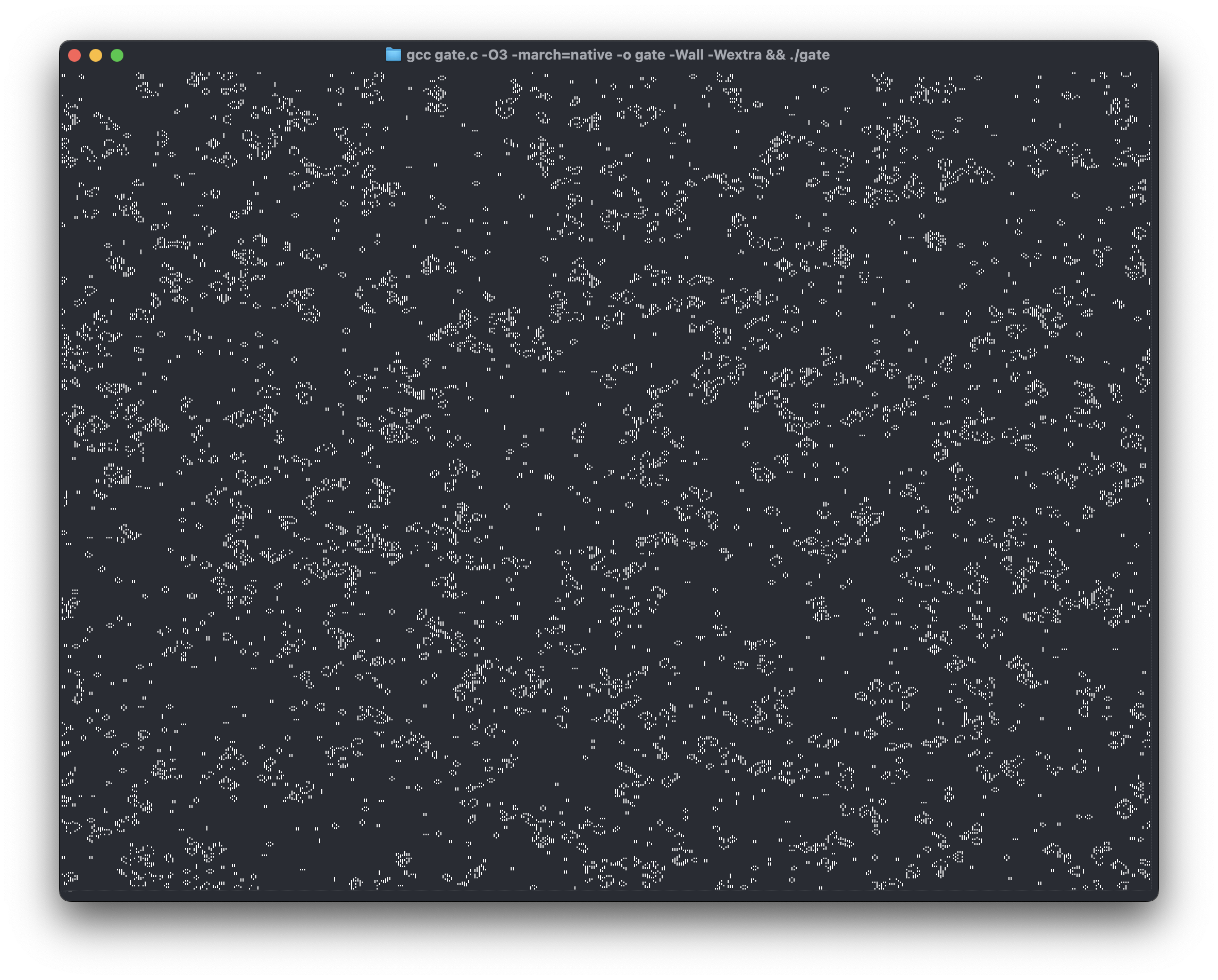
(Please don’t kill me for writing thousands of words about Conway’s Game of Life without a single picture or animation; I know, I’m working on it. Update: added a 600kb picture LOL. Animation coming soon.)
Thank you to Shaw, Anthony, Mike, Clara and friends for taking a look, fixing typos, and providing feedback/moral support while I worked on difflogic.
What's Your Reaction?
 Like
0
Like
0
 Dislike
0
Dislike
0
 Love
0
Love
0
 Funny
0
Funny
0
 Angry
0
Angry
0
 Sad
0
Sad
0
 Wow
0
Wow
0