Multiplatform Matrix Multiplication Kernels

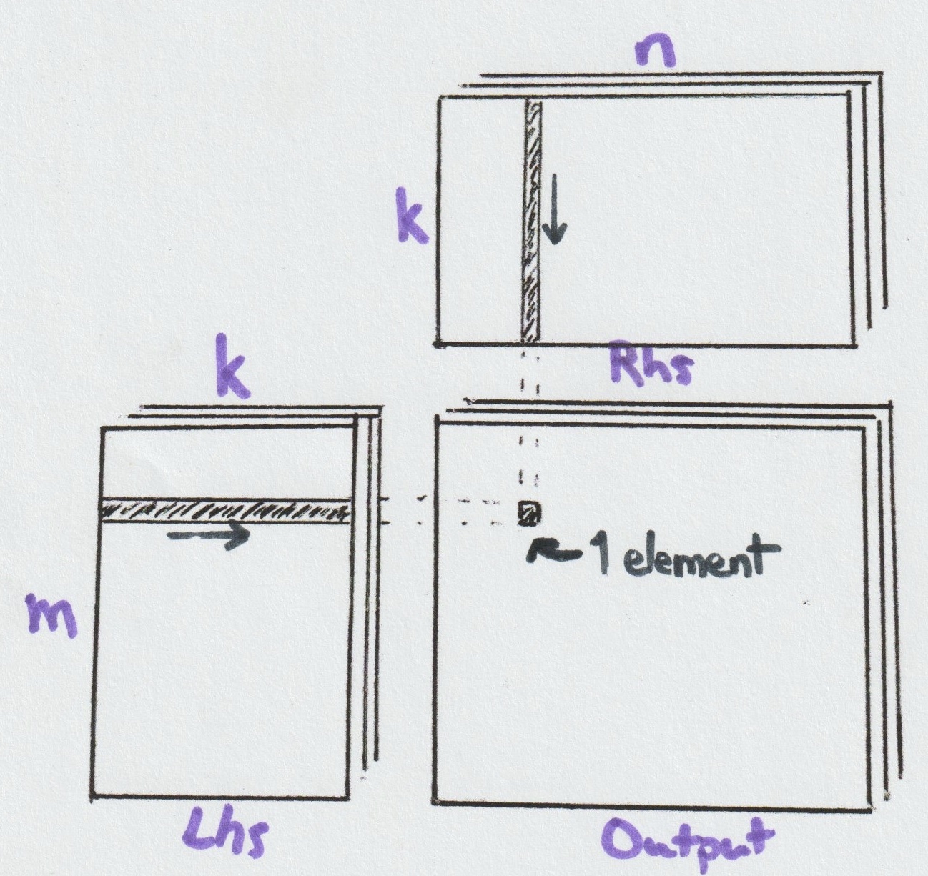
Let's set aside batching and focus on the core problem of computing the matrix product Lhs × Rhs with shapes [m, k] × [k, n], which we'll refer to as an (m, n, k)-Matmul.

A naive CPU implementation would iterate over the m and n dimensions, computing dot products along k for each (m, n) pair. As illustrated in the above figure, each output element results from a dot product (or inner product) involving k multiply-add operations. This process is repeated m × n times—once for each output element.

The same result can also be computed as a sum of k outer products. An outer product is what you get when you multiply a column vector by a row vector — it gives you all combinations of their elements, filling an entire matrix. This approach requires maintaining all m × n intermediate results (accumulators) at once, but avoids reloading the same data multiple times. Quite interestingly, we will actually use both strategies, depending on the level of tiling.

Complexity

A matrix multiplication consists of m × n dot products, each involving vectors of length k. Each dot product requires k multiply-and-add operations, which modern hardware can often fuse into single instructions. Although the Strassen algorithm can theoretically reduce the number of operations, its practical implementation usually results in fewer fused multiply-add instructions, making it less efficient in practice [8]. Therefore, we consider 2 × b × m × n × k as the fundamental operation count. Dividing this operation count by execution time yields the achieved number of TFLOPs, a measure we will use in the benchmarks section to compare our algorithms.

This means that given optimal hardware instruction usage, there exists a theoretical performance ceiling. Our goal in optimizing Matmul at the software level is to approach this ceiling as closely as possible. In other words, matrix multiplication is compute-bound, and our challenge lies in minimizing or hiding global memory access latency.

As we've discussed in our previous explorations of quantization [9] and fusion techniques [4], global memory access almost always represents the primary performance bottleneck in GPU computing. While several optimization strategies exist - including memory coalescing, vectorization through SIMD loads, and efficient unit grouping with planes - implementing these optimizations requires careful consideration. Simon Böhm's excellent analysis of CUDA matrix multiplication [10] provides a thorough progression through some of these optimization techniques. However, without disciplined, continuous refactoring, you'll likely find yourself maintaining a monolithic, overwhelmingly complex kernel. This reality led us to develop a more structured approach using CubeCL.

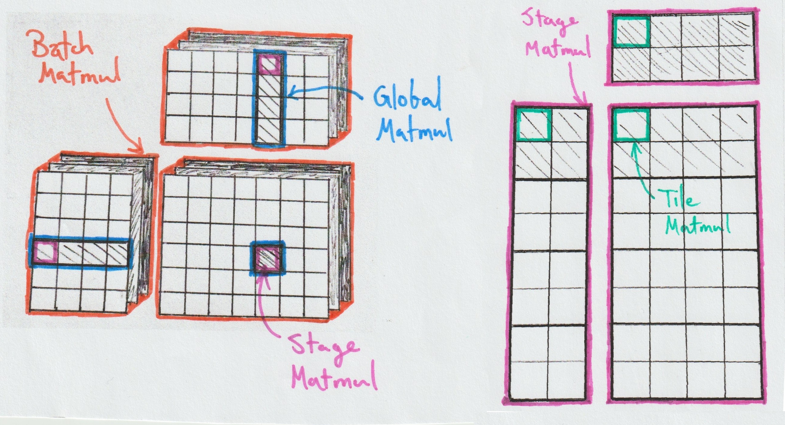
Four Levels of Abstractions

CubeCL's Rust-based approach to GPU programming leverages traits and generics to encode multiple matrix multiplication implementations through composable components, using abstractions that incur zero runtime cost. The architecture divides matrix multiplication into four distinct levels, each handling progressively larger problem scales using a divide-and-conquer strategy. This hierarchical structure makes it possible to split a single Matmul into smaller, more manageable Matmuls, optimizing data locality and movement at each level:

1. Tile Matmul: Interfaces directly with hardware capabilities
2. Stage Matmul: Manages shared memory operations for local computations
3. Global Matmul: Accumulates results from a series of Stage Matmuls over arbitrary k dimensions
4. Batch Matmul: Orchestrates multiple Global Matmuls across the entire computation

The power of CubeCL lies in its type system, which enables arbitrary composition of these levels. For instance, our Global Matmul implementations are generic over Stage Matmuls, and so on. Unlike cuBLAS, we don't rely on pre-compiling every variant—instead, JIT compilation handles specialization on the fly and, thanks to techniques we outlined in a previous post [11], this remains fast even for complex strategies.

Plane vs Unit

As we hinted earlier, we'll almost exclusively treat the plane as our finest primitive of computation. The Batch Matmul doesn't even deal with anything below Cubes, and the Global Matmul is responsible for ensuring memory coalescing when loading data — so it operates strictly at the plane level. At deeper levels, where memory access is no longer a bottleneck, the Stage and Tile Matmuls can be configured to work either at the plane or unit level, with minimal architectural impact but significant performance implications.

In the next two sections, we'll focus on plane-level Matmuls for simplicity, though unit-level versions also exist.

Tile Matmul: The Low-Level Instruction

The Tile Matmul layer operates at the lowest level, handling the fundamental multiply-and-add operations.

In the above figure, the instruction corresponds to a (8, 8, 8)-Matmul — a choice made for readability that aligns with acceleration supported by Apple's Metal framework. This contrasts with modern NVIDIA GPUs, where specialized hardware units called Tensor Cores perform matrix multiplication using larger tiles such as (16, 16, 16). Tensor Cores deliver highly optimized performance and process up to 256 dot products simultaneously, though only a few tile shapes are supported [12].

As software developers, competing with Tensor Core performance is quite futile — except in specific cases, such as degenerate input shapes or when accelerators are unavailable. Our focus should be to maintain a steady flow of data to the Tensor Cores to keep them fully utilized.

As a result, the most effective approach is often the simplest: directly calling the underlying accelerator API. In such cases, this Matmul level essentially reduces to issuing simple instructions per plane, executed collectively by all its units. Here's what the (simplified) trait looks like [7]:

pub trait TileMatmul {
    type LhsTile;
    type RhsTile;
    type Accumulator;

    fn init_lhs() -> Self::LhsTile;
    fn init_rhs() -> Self::RhsTile;
    fn init_accumulator() -> Self::Accumulator;
    fn reset_accumulator(acc: Self::Accumulator);

    fn load_lhs(tile: Self::LhsTile);
    fn load_rhs(tile: Self::RhsTile);

    // Execute the Matmul of lhs and rhs and adds it to acc. 
    fn execute(lhs: Self::LhsTile, rhs: Self::RhsTile, acc: Self::Accumulator);
}
  

You may have noticed that, even after the sum of outer products, the final result of the execution is not just stored in an output — it is added to a given accumulator. This will be essential when dealing with larger Matmuls.

The tiles are typically stored in registers, which — as mentioned earlier — can significantly impact occupancy and increase stalls. To mitigate this, we can use double buffering, introducing enough independent instructions between the global memory fetch and the use of the fetched data. This is normally handled inside the next abstraction.

What About GPUs Without Tensor Cores?

That's a good question — but it also applies to any matrix multiplication that doesn't map cleanly to the instruction sizes supported by tensor cores. This includes operations like outer products, inner products, matrix-vector and vector-matrix multiplications — that is, (m, n, 1), (1, 1, k), (m, 1, k), and (1, n, k)-Matmuls. For these cases, you can use a unit-level Tile Matmul, which is conceptually close to a simple triple for-loop implementation, and where the instruction size is almost fully dynamic.

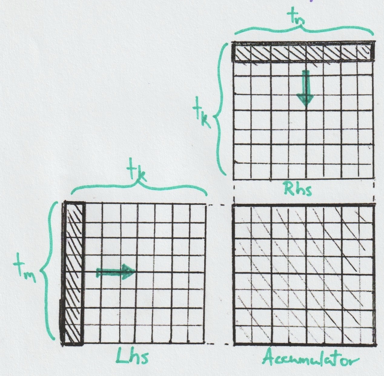
Stage Matmul: Partitioning over Planes

The Stage Matmul sits at the center of our abstraction pipeline and therefore has a significant impact. Its main role is to coordinate the work of underlying Tile Matmuls by specifying which tiles in shared memory they should operate on. The actual loading into registers is handled by the Tile Matmuls themselves, for each plane (or each unit).

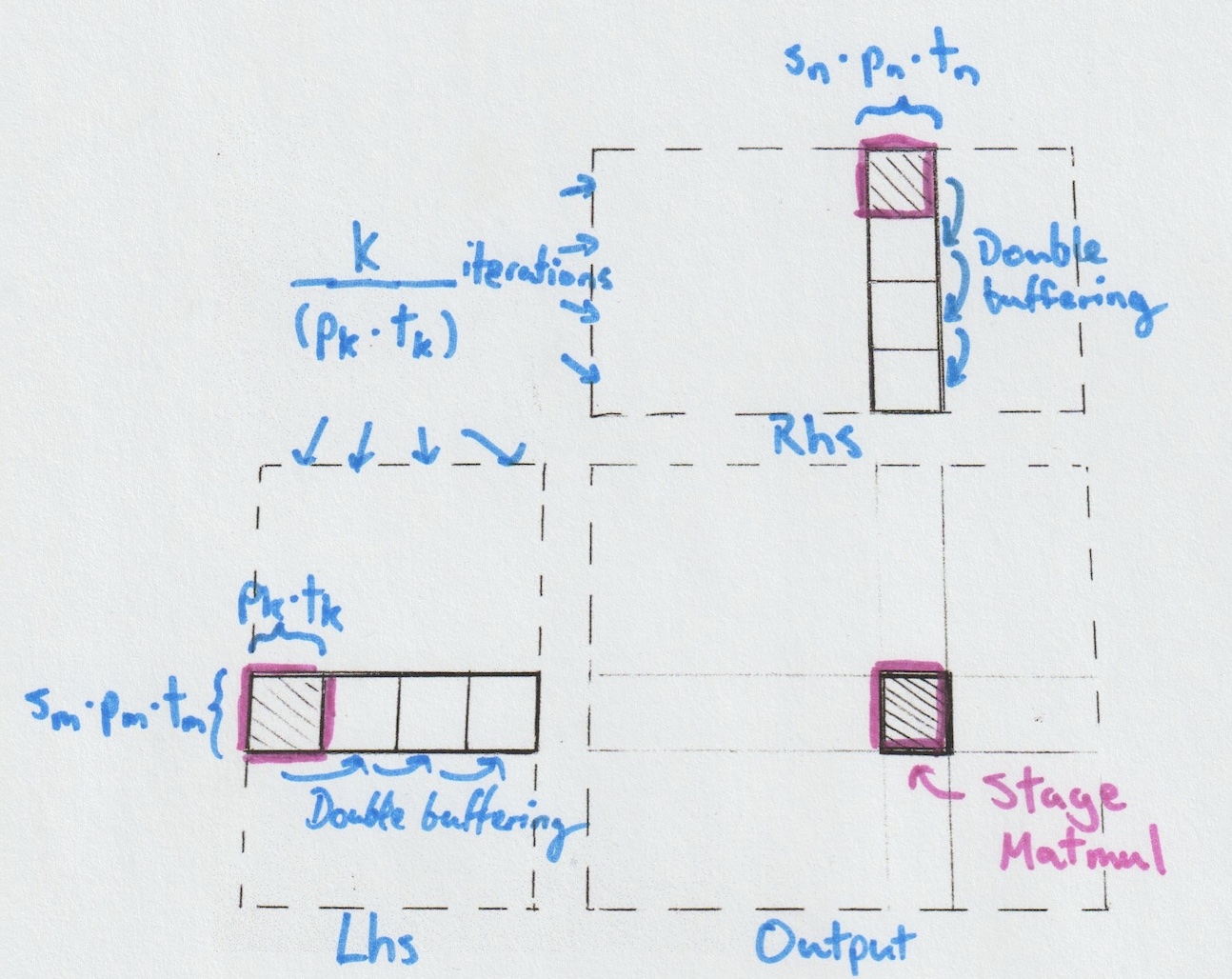
Since we assume shared memory is already pre-loaded with inputs, and the underlying Tile Matmul is responsible for loading them into registers, this Matmul level doesn’t perform data movement itself. Instead, its role is to determine which m tile of Lhs and n tile of Rhs should be read, and by which plane. Each (m, n) pair’s result will be added to an existing accumulator, which enables looping over p_k.

As we'll see in the Global Matmul section, the Stage Matmul is used multiple times to perform complete reductions. But why have p_k > 1 if the Global Matmul ensures the completion of the reduction? It's a tradeoff: it lets us offload more reduction work into each Stage Matmul, saving on the overhead of additional Global Matmul iterations—at the cost of needing more shared memory.

Similarly, we can adjust s_m, p_m, _sn, and p_n to balance tradeoffs between shared memory size (the sizes of Lhs and Rhs in the figure above) and register usage for one Cube (the size of the accumulator). But be aware: these configurations also affect the number of Cubes and planes launched. Everything is interconnected, making the tradeoffs delicate.

Let us now look at the StageMatmul trait. The most curious artifact is the StageEventListener, which allows higher-level Matmuls to inject arbitrary instructions into the Stage Matmul implementation. It's a compilation-time mechanism that simply results in some lines of code cleverly inserted between Tile Matmul executions. This will be useful later on.

pub trait StageMatmul {
    /// Readers can read a tile from shared memory
    type LhsReader;
    type RhsReader;
    /// Collection of Tile Matmul accumulators
    type Accumulator;
    /// Defines how to write to output
    type Writer;

    fn init_accumulator() -> Self::Accumulator;

    /// The listener allows injecting Global Matmul actions between any event
    /// happening inside the Stage Matmul. In practice, it helps interleaving 
    /// loading with execution. 
    fn execute<L: StageEventListener>(
        lhs: Self::LhsReader,
        rhs: Self::RhsReader,
        acc: Self::Accumulator,
        listener: L,
    );

    /// Writing to the output is the responsibility of the Stage Matmul,  
    /// since it holds the computed results in its accumulator.
    fn write_results(acc: Self::Accumulator, out: Self::Writer);
}
  

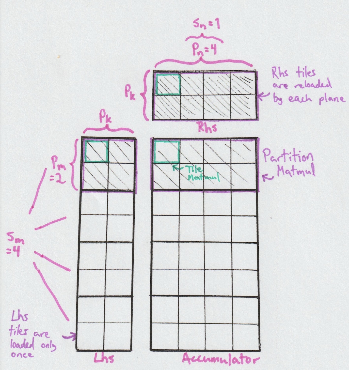
Partition Matmul

Inside our Stage Matmul implementations, we use s_m × s_n planes. By fixing s_n=1 as in the figures, we then have s_m planes, each reading p_m independant rows of Lhs, but sharing the same p_n columns of Rhs. This sub-matmul specific to one plane is called a Partition Matmul.

In such cases, where rows of Lhs are needed by only one plane, we can actually ask the planes to load from global memory straight to registers and skip the need for an Lhs shared memory, but this comes with a set of assumptions. We call those algorithms Ordered because they need to be more careful with the order in which they overwrite their registers.

What happens inside a Partition Matmul is simply an outer product over Tile Matmuls. For a fixed k in [0, p_k), we execute all combinations of tiles from Lhs with tiles from Rhs. When fetching data from shared memory to registers, the potential for a stall is real. To avoid that we use an extra tile for Rhs, double buffering as we advance through p_n. Notably, this stall is a good opportunity to perform unrelated work, such as injecting Global Matmul instructions via the StageEventListener.

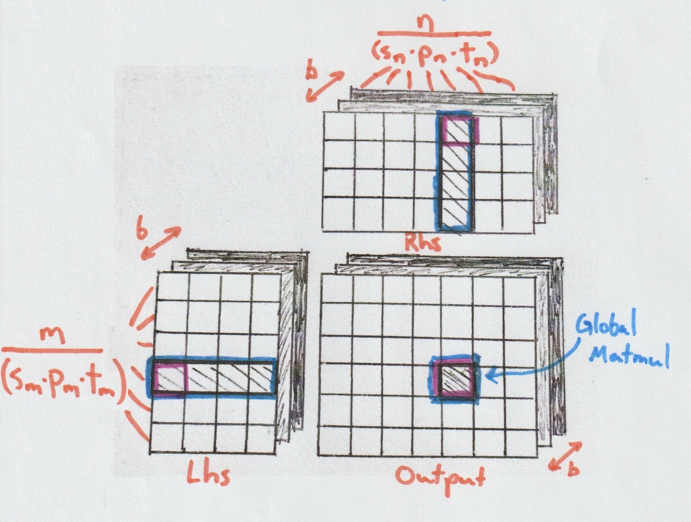
Global Matmul: Accumulating Full Dot Products

The role of the Global Matmul is to loop over the input tiles along the reduction dimension, fetching data from global memory and storing it in shared memory. Each tile is then fed into the underlying Stage Matmul, which performs partial accumulation. Once all tiles have been processed, the final result is written back to global memory.

A single Cube can perform this operation independently, computing complete dot products for its assigned portion of the input tensors. If k is not divisible by p_k × t_k, the Global Matmul will need to perform bound checks—conditional instructions that introduce branching within planes and slow things down. For this reason, it's generally good practice, when possible, to choose problem sizes and stage configurations that divide evenly.

Let's take a look at the (simplified) trait.

pub trait GlobalMatmul {
    /// Loaders can read global memory and write it to shared memory. 
    type LhsLoader;
    type RhsLoader;

    /// Typically the same as those of the underlying Stage Matmul
    type Accumulator;
    type Writer;

    fn init_lhs_loader() -> Self::LhsLoader;
    fn init_rhs_loader() -> Self::RhsLoader;
    fn init_accumulator() -> Self::Accumulator;

    fn execute(
        lhs_loader: Self::LhsLoader,
        rhs_loader: Self::RhsLoader,
        writer: Self::Writer,
        acc:  Self::Accumulator,
    );
}
  

Similar to the Stage Matmul, stalls can also occur here because writing to shared memory requires loading data from global memory into registers. To avoid these stalls, we can apply the previously explained double buffering approach—just at a different level. Another option is to use custom instructions to program specialized embedded units designed for this purpose. NVIDIA introduced TMA (Tensor Memory Accelerator) [13] to optimize exactly that!

To make our approach portable across different GPUs, we define a loader, which specifies how global memory is fetched and written to shared memory. Among the loader strategies we explored, the two most effective were:

• Cyclic: Suppose there are 64 × 16 = 1024 elements to load to Lhs. Without regards to underlying tiles or partitions, we use every unit at our disposal, in order, to load one piece of data, then they start again with an offset. Given 4 planes of 32 units, this would take 1024 / (4 × 32) = 8 loading tasks for each unit.
• Tilewise: Each plane cycles by itself over the partition where it will perform compute. This has practical implications, in that it doesn't need to sync with other planes before starting to compute.

In our simpler Matmul implementations, each plane is responsible for both loading data and performing computation. In some algorithms, however, we use a technique called specialization, where different planes are assigned distinct tasks. It's important not to apply specialization within a single plane, as that would introduce costly branching and significantly degrade performance.

Why would we use plane specialization? Primarily, to optimize the hardware resources mentioned earlier. By dedicating certain planes solely to computation and others to data loading, we can better manage register usage — which is dominated by the accumulators in compute planes. Therefore, load-only planes help increase SM occupancy without adding significant register pressure.

Batch Matmul: Dispatching over SMs

The Global Matmul can solve problems with arbitrarily large k using a single Cube, but it is still limited to fixed m and n. Put otherwise, it computes only a small rectangle of the final output. To cover the entire result, we need another level of abstraction: the Batch Matmul, which handles the dispatch over all those small rectangles.

This is the simplest trait in the hierarchy and serves as the entry point to the Matmul kernel, which is why it operates directly on tensors. As mentioned at the beginning, the whole reason for having a custom Matmul implementation is to enable fusion. So how does fusion fit into this? With CubeCL, we use a VirtualTensor, a type of tensor that abstracts a block of computation resulting in a value being read or written. This allows us to write the algorithm and configure the virtual tensor to behave much like a normal global tensor, with fusion performed on both reads and writes. For more on fusion, see our earlier post [4].

pub trait BatchMatmul {
    fn execute(
        lhs: VirtualTensor,
        rhs: VirtualTensor,
        out: VirtualTensor,
        cube_count_plan: CubeCountPlan,
    );
}
  

Dispatching Cubes to compute correct results is straightforward, but achieving optimal performance requires some care. Since neighboring computations often share input data — for example, computations in the same row reuse the same Lhs tiles — thoughtful scheduling can improve L2 cache reuse. The goal is to help the GPU scheduler assign work to SMs in a way that increases the likelihood of cache hits. We can influence this behavior by controlling a few key parameters:

• Given a Cube index from 0 to 41, to which rectangle should it map to? We have the strategies Row- and Col-Major, as well as Swizzle Row- and Swizzle Col-Major. Swizzle maps a linear index to 2D coordinates by zigzagging through strips in alternating directions, so each new coordinate reuses data recently visited. Here's how Swizzle Row-Major would dispatch the Cube indices for the example in the figure:

  ┌────┬────┬────┬────┬────┬────┬────┐ 
  │  0 │  3 │  4 │  7 │  8 │ 11 │ 12 |
  ├────┼────┼────┼────┼────┼────┤────┤ 
  │  1 │  2 │  5 │  6 │  9 │ 10 │ 13 |
  ├────┼────┼────┼────┼────┼────┤────┤ 
  │ 26 │ 25 │ 22 │ 21 │ 18 │ 17 │ 14 |
  ├────┼────┼────┼────┼────┼────┤────┤ 
  │ 27 │ 24 │ 23 │ 20 │ 19 │ 16 │ 15 |
  ├────┼────┼────┼────┼────┼────┤────┤ 
  │ 28 │ 31 │ 32 │ 35 │ 36 │ 39 │ 40 |
  ├────┼────┼────┼────┼────┼────┤────┤ 
  │ 29 │ 30 │ 33 │ 34 │ 37 │ 38 │ 41 |
  └────┴────┴────┴────┴────┴────┴────┘
  

• Given 42 Cubes to launch, how should they be dispatched across the CubeCount's x, y, and z coordinates? Based on our experience, the best results come from setting y to the number of SMs and x to the number of cubes per SM. However, many hardware configurations have inconvenient SM counts—like 19 or 46—which can lead to extra, unused cubes. In practice, it can therefore be better to use a common divisor of the number of SMs and the number of Cubes needed to achieve a more balanced distribution.

What They Don't Tell You

Obviously, when explaining our architecture, we left out many important details that are crucial to attain state-of-the-art performance. In particular, there are many things not explicitly documented that we had to discover on our own, and conversely, some overemphasized topics that didn't really matter.

Registers

• Accumulators reside in registers and persist throughout the entire execution of the Global Matmul, despite being defined by the Tile Matmul. Achieving this elegant abstraction would be extremely challenging without Rust's associated types — otherwise, we'd likely have to revert to a pointer-based approach.

• Since accumulators reside in registers for the entire duration of the computation, requesting too many registers can cause spilling into much slower memory. Accumulator size is directly tied to the m and n parameters of the stage, partition, and tile, imposing an implicit limit beyond which performance is significantly penalized.

Double buffering

• What exactly are buffers in the double buffering approach? While it's clear that there should be double buffering at both Global and Stage levels [14], some details had to be inferred through experimentation. At the Stage level, we found we had to declare an extra tile only for Rhs and double buffer inside a partition. At the Global level, we made shared memory twice as large as p_k × t_k, using a single contiguous region and alternating between its two interleaved halves, rather than allocating separate shared memory buffers.

• Double buffering relies on asynchrony, i.e. the ability to overlap computation with memory operations But it is unclear how to induce asynchrony, we need a way to ensure that compute could proceed without blocking on memory loads. What proved effective was interleaving Global loading tasks between Tile Matmuls of the same partition. That kind of broke our abstractions at first, leading to the introduction of the StageEventListener, a mechanism to inject code between different levels. This proved to be a powerful tool.

Lines

• In the previous discussion on loaders, we skipped an important detail: vectorization, what we refer in CubeCL as lines. Rather than loading a single float at a time, CubeCL operates on lines of floats using SIMD instructions. The maximum line size depends on the hardware and how cleanly the problem shapes divide.

  Earlier, in the cyclic loader example, we mentioned loading 64 × 16 = 1024 elements into Lhs using 4 × 32 = 128 units, resulting in 1024 / 128 = 8 loading tasks per unit. But that ignored vectorization. With a line size of 8, for instance, each unit would only need to perform a single task. In practice, that might not be enough tasks to fully hide memory latency and trigger asynchronous behavior, but the example is intentionally small, it becomes a heavier workload with tile sizes such as (16, 16, 16).

• Very interestingly, when writing to shared memory in a vectorized fashion, it naturally distributes memory transactions across banks and eliminates the need for explicit padding [15]. Therefore, contrary to common advice, we found that no additional padding was necessary in shared memory.

Tensore Core Data Layout

• A detail that's often glossed over is the change in layout between global and shared memory. For example, while entire tensors might be stored in row-major order in global memory, we store tiles in shared memory contiguously. For instance, all elements of an 8 × 8 tile are laid out back-to-back before moving to the next tile. Although strided layouts are possible, we found that fully contiguous tiles offered slightly better performance. It's best to handle the layout adjustment within the loaders.

• What's more confusing is what happens once the data moves into registers for Tensor Core computation. At that point, we only know that the data for a given tile resides somewhere within a plane's registers. In practice, each unit holds a portion of that plane, but the exact mapping is opaque. This ambiguity doesn't affect computation: the Tensor Core API guarantees that once the tile is loaded, the instructions will execute correctly, regardless of the internal layout.

  However, this black-box behavior becomes a problem after all computations. Sure, the plane holds the result of all the dot products for a tile's worth of output elements—but we need to write those results back to global memory in the correct positions. The Tensor Core API provides a cooperative store operation that writes all data in row-major order, but this doesn't match our global tensor layout directly. Mirroring how we reshaped data when loading into shared memory, we now have to map it back—but this time without knowing which unit holds which part. The most efficient solution we found was to store into an intermediate shared memory, then have units re-read it in a deterministic way to store every element to its right spot.

Different Algorithms

Now that we've introduced the different levels of abstraction, explained why they exist, and discussed the key caveats to keep in mind when writing matmuls, we can look at how these components come together to form full algorithms. To support this, we defined the Algorithm trait, which is responsible for composing the building blocks, declaring their assumptions, and providing a way to configure them. Again, we show a simplified version here for readability.

pub trait Algorithm {
    type TileMatmul: TileMatmulFamily;
    type StageMatmul: StageMatmulFamily;
    type GlobalMatmul: GlobalMatmulFamily;
    type BatchMatmul: BatchMatmulFamily;

    fn setup<MP: MatmulPrecision, R: Runtime>(
        client: &ComputeClient<R::Server, R::Channel>,
        problem: &MatmulProblem,
        selection: &MatmulSelection,
        line_sizes: &MatmulLineSizes,
    ) -> Result<<Self::BatchMatmul as BatchMatmulFamily>::Config, MatmulSetupError> {
        Self::BatchMatmul::setup::<MP, R>(client, problem, selection, line_sizes)
    }

    fn selection<R: Runtime>(
        client: &ComputeClient<R::Server, R::Channel>,
        problem: &MatmulProblem,
    ) -> MatmulSelection;
}

Each algorithm is actually a family of kernels, configurable through tile size, partitioning, stage size, and other advanced parameters.

1. Simple. This one is surprisingly good on certain GPUs and configurations. Instead of relying on software pipelining (double buffering), it relies on minimizing register pressure with a heavy partitioning of Lhs, therefore improving occupancy.

   Tensor Cores	✅
   Double Buffering	❌
   Ordered Loading	❌
   Plane Specialization	❌

2. Simple Multi Row. Like the Simple algorithm, but growing p_m > 1, incurring less partitioning and more responsibility to each plane.

   Tensor Cores	✅
   Double Buffering	❌
   Ordered Loading	❌
   Plane Specialization	❌

3. Simple - Unit. Very similar to the Simple: When the Tile Matmul is implemented without the use of custom instructions to leverage Tensor Cores, it can be better to improve occupancy rather than software pipelining. With smaller underlying tiles, we can reduce the number of registers used for storing accumulators. Coupled with heavy Lhs partitioning, we can get impressive performance even without Tensor Cores. For Outer product, that algorithm normally outperforms kernels in cuBLAS by a significant amount. Compared to the non-Tensor Core implementation used in earlier versions of Burn, this approach can deliver up to 3 times better performance. This improvement itself is very significant, especially for neural networks deployed on the web using wgpu, where Tensor Cores can't be used.

   Tensor Cores	❌
   Double Buffering	❌
   Ordered Loading	❌
   Plane Specialization	❌

4. Double Buffering. The double buffering algorithm typically uses the double-buffered variants of both the Global and Stage Matmul traits. Its primary goal is to reduce stalls through software pipelining rather than by optimizing resource usage. It's also highly configurable. For example, we can control specialization by defining the responsibility of each plane involved in the computation. Overall, this algorithm performs well but is resource-intensive and may not run smoothly on all GPUs. Due to its high register usage, it generally avoids partitioning Lhs, as doing so would further increase register pressure.

   Tensor Cores	✅
   Double Buffering	✅
   Ordered Loading	❌
   Plane Specialization	❌

5. Double Buffering Unit. Like the Simple Unit, but with double buffering activated.

   Tensor Cores	❌
   Double Buffering	✅
   Ordered Loading	❌
   Plane Specialization	❌

6. Double Buffering Specialized. As mentioned earlier, adding plane specialization to double buffering can improve resource efficiency by separating compute and load tasks, which reduces register pressure and increases SM occupancy.

   Tensor Cores	✅
   Double Buffering	✅
   Ordered Loading	❌
   Plane Specialization	✅

7. Double Buffering Ordered. The Double Buffering Ordered is similar to the Double Buffering algorithm, but the specialization and loader of Lhs aren't configurable. This is by design: by carefully ordering ordering memory loads, we can eliminate the need for synchronization between loading planes and skip shared memory for one of Lhs's stages entirely, loading it directly into registers. This may seem like a minor optimization, but when combined with aggressive Lhs partitioning—which increases Lhs memory pressure—it can perform exceptionally well on certain GPUs.

   Tensor Cores	✅
   Double Buffering	✅
   Ordered Loading	✅
   Plane Specialization	❌

Preliminary Benchmarks

Below are benchmarks of kernels generated by our matrix multiplication engine, grouped by hardware. For simplicity, all problem shapes are square. Throughput is reported in TFLOPs, computed as:

TFLOPs = (2 × b × m × n × k) ÷ (time × 10¹²)

where b is the batch size, m, n, and k are matrix dimensions, and time is the execution time in seconds. Higher TFLOPs indicate greater utilization of tensor cores for computation, less time spent waiting on memory, thus a more efficient algorithm overall.

Let's go through a few caveats before we begin:

• For these benchmarks, we only included kernel variants that use tensor cores. We excluded the Unit variants, as comparing them directly would be unfair. They can outperform tensor-core variants on small shapes or special cases, which are not covered here.

• CubeCL's compiler infrastructure still needs improvement, and some performance limitations lie outside the matmul engine itself. For example, due to a constraint in the Vulkan compiler, all Vulkan benchmarks use a line size of 4, whereas other backends use 8 on the same benchmarks. Similarly, HIP compiler for ROCm has unresolved issues at the time of writing.

• Algorithms are highly configurable, making parameter selection a nontrivial task. Our aim isn't to find a single configuration that works for everything, nor to fine-tune each shape and device individually. Instead, we rely on a heuristic that adapts to problem shapes across platforms, reducing the need for full autotuning. This heuristic is still evolving and occasionally produces suboptimal results.

• We only have a reference point on the CUDA benchmarks, because all matmuls are executed through Burn, which only exposes non-CubeCL state-of-the-art implementations for CUDA. Smaller shapes (up to 4096³) launch a cuBLAS kernel, while larger ones launch a CUTLASS kernel. The other figures are still useful to understand how the different algorithms compare.

• The devices used for benchmarking are our team's developer machines. In the future, we plan to provide official benchmarks on more standardized hardware.

NVIDIA

AMD

Apple Silicon

You Can Help Us

While we’ve achieved state-of-the-art performance in certain contexts, further work is needed to generalize it across all scenarios. Head over to the Burn Community Benchmarks to upload your results, and feel free to experiment with the matmul bench code to discover better configurations.

References

[1]Becoming the Fastest: Introduction[2]cuBLAS[3]NVIDIA cuDNN[4]Optimal Performance without Static Graphs by Fusing Tensor Operation Streams[5]CUTLASS: Fast Linear Algebra in CUDA C++[6]CubeCL: Multi-platform high-performance compute language extension for Rust.[7]CubeCL-Matmul[8]Matrix Computations, by Gene H. Golub and Charles F. Van Loan (4th edition, 2013).[9]Why Quantization Matters[10]How to Optimize a CUDA Matmul Kernel for cuBLAS-like Performance: a Worklog[11]Improve Rust Compile Time by 108X[12]CUDA C++ Programming Guide: Element Types and Matrix Sizes[13]CUTLASS Tutorial: Mastering the NVIDIA® Tensor Memory Accelerator (TMA)[14]Efficient GEMM in CUDA[15]LU, QR and Cholesky Factorizations using Vector Capabilities of GPUsWhat's Your Reaction?